Chapter 11 Result and Validation
11.1 Calculation of Total Weightage
Sum weightage for all the parameter classes to obtain the total weightage for each cell of the raster data. In order to do this, we need to reclassify the raster again according to the weightage.
Let us consider the weightage for slope we calculated in last chapter.
| Slope Class | Landslide Area(\(m^2\)) | Total Area(\(m^2\)) | Weightage |
|---|---|---|---|
| 1 | 0.00 | 11055469 | -23.0574 |
| 2 | 18750.00 | 50373750 | -0.9195 |
| 3 | 57968.75 | 43957344 | 0.3455 |
| 4 | 18281.25 | 4650469 | 1.4377 |
| 5 | 7812.50 | 100625 | 4.4209 |
Weightage for slope class 1 = -23.0573670
We reclassify all the slope class with value 1 to -23.0573.
To reclassify the slope class raster, we again create rules file slopewtrule.txt as follows:
1:1:-23.0574:-23.0574
2:2:-0.9195:-0.9195
3:3:0.3455:0.3455
4:4:1.4377:1.4377
5:5:4.4209:4.4209
In the similar way, we calculate rules for each parameters using r.recode as before.
After we reclassify all the raster-weightage file, we will find the sum.
Summation of all the raster-weightage file is simple. Use the following code:
r.series input=aspectwt,slopewt,ndviwt,ndwiwt,profwt,tanwt,riverwt output=sumwt method=sum
Where each input corresponds to the weightage for each parameter and sumwt is the output raster.
Read the manual for r.series and you will find that it can be used to calculate various statistics from multiple rasters.
The summed weightage raster is shown in the following image.
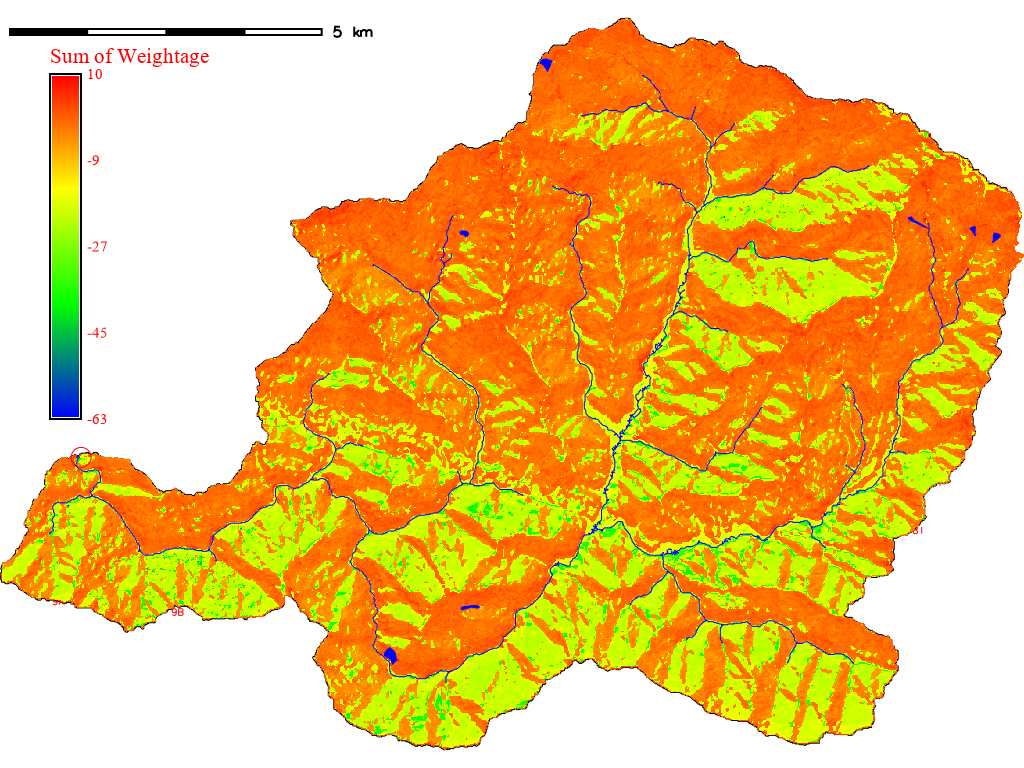
Figure 11.1: Sum of weightage of all parameters
Beyond this, you will need personal judgement and sum reading of references. However, it is always possible to refer to the same process as explained below.
Final product of landslide susceptibility analysis is a raster data classified into susceptibility ranges, e.g., high hazard, moderate hazard, low hazard etc. To do this we will follow the steps below:
- Find the distribution of weightage (quantile), that is, area corresponding to each weightage range.
- Reclassify the sum of weightage into these ranges.
- Find the areas of landslide in each quantile ranges.
- Find the success rate for prediction.
- Select the boundary values for classifying the hazard level.
11.2 Distribution of sum-of-weight
Run the following code to find the distribution of weightage sum.
r.quantile -r input=sumwt@PERMANENT quantiles=100 file=path/to/sumwtquantile.txt
The above code will distribute the range into 1% interval by area. The flag -r creates a rules file for reclassification. The output will be saved as sumwtquantile.txt.
-77.666700:-53.535600:1
-53.535600:-51.016200:2
-51.016200:-36.618101:3
-36.618101:-35.991301:4
-35.991301:-35.368399:5 and so on
The above quantile distribution means that sum of weightage from -77.7 to -53.5 occupies 1% of the whole area of the region and so on.
11.3 Reclassify the Weightage Sum
Use the rules file and use r.recode to reclassify the raster.
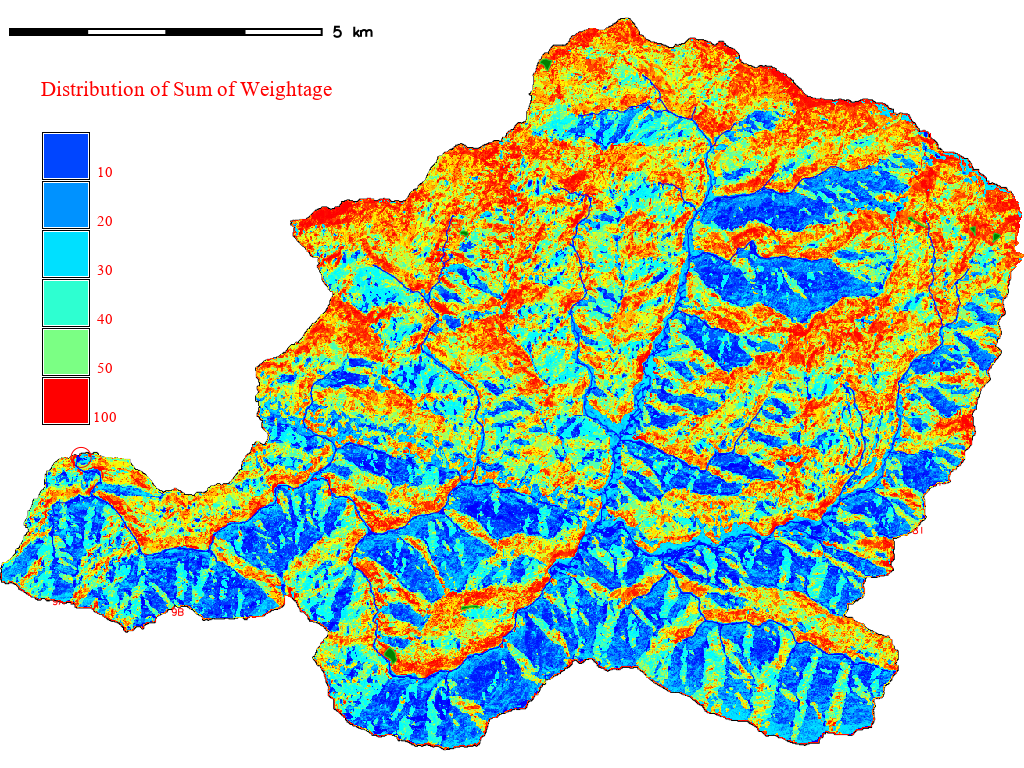
Figure 11.2: Quantile Distribution of Sum of Weightage
11.4 Find the Area of Landslide in Each Quantile Range
Let us again use the r.stats code to to find the distribution of landslide in each range.
- Code to calculate stats:
r.stats -a –overwrite input=wtqantile,lsrast output=path/to/sumwtcross.csv separator=, null_value=-1 - Open output file sumwtcross.csv.
| Sum of Weight Class | Landslide | Area(\(m^2\)) |
|---|---|---|
| 1 | -1 | 1111718.8 |
| 2 | -1 | 1110937.5 |
| 3 | -1 | 860000.0 |
| 4 | -1 | 1307031.2 |
| 5 | -1 | 1162343.8 |
| 6 | -1 | 1099531.2 |
| 7 | -1 | 1223281.2 |
| 8 | -1 | 1127343.8 |
| 9 | -1 | 991406.2 |
| 10 | -1 | 1113125.0 |
| Sum of Weight Class | Landslide | Area(\(m^2\)) |
|---|---|---|
| 95 | -1 | 1106406.25 |
| 96 | 1 | 5468.75 |
| 96 | -1 | 1075312.50 |
| 97 | 1 | 12031.25 |
| 97 | -1 | 1105312.50 |
| 98 | 1 | 7656.25 |
| 98 | -1 | 1124687.50 |
| 99 | 1 | 16718.75 |
| 99 | -1 | 1090937.50 |
| 100 | 1 | 19375.00 |
| 100 | -1 | 1093750.00 |
11.5 Find the success rate
Success rate of the sum of weightage is determined by how many percentage of landslide are predicted by the highest sum of weightage. Let us see the area of landslide within each of the top sum-of-weightage class.
| Percentage Map | Percentage Landslide Area |
|---|---|
| 0 | 0.00000 |
| 1 | 18.84498 |
| 2 | 35.10638 |
| 3 | 42.55319 |
| 4 | 54.25532 |
| 5 | 59.57447 |
| 6 | 64.43769 |
| 7 | 70.36474 |
| 8 | 71.73252 |
| 9 | 73.55623 |
Above table shows the cumulative area of landslide within each percentile starting from highest weightage. We can see that area of landslide within top 1% of the pixels = \(19375.00m^2\), which is about 19% of the total area. Similarly, area of landslide within top 2% is about 35%. Plotting the values of cumulative landslide area with respect to the percentile will give us the idea of success rate of the susceptibility map. Following image shows the graph of success rate.
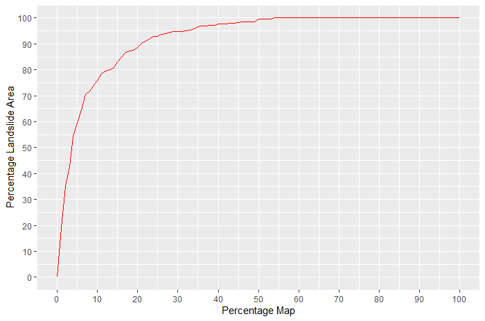
Figure 11.3: Success Rate of Prediction
11.6 Select the Boundary Value for Hazard Zone
We can observe following points from the above graph:
- About 90% of landslides occur in the top 20 percentiles.
- About 100% of landslides occur in the 50 percentiles.
- Bottom (Lowest sum-of-weightage) 50% has no landslide.
We will chose the boundaries between three hazard zones and reclassify the quantile raster again into landslide classes using the following rule:
1:50:1
51:80:2
81:100:3
Where 1, 2 and 3 represent low, moderate and high hazard respectively.
With this we get the final susceptibility map.
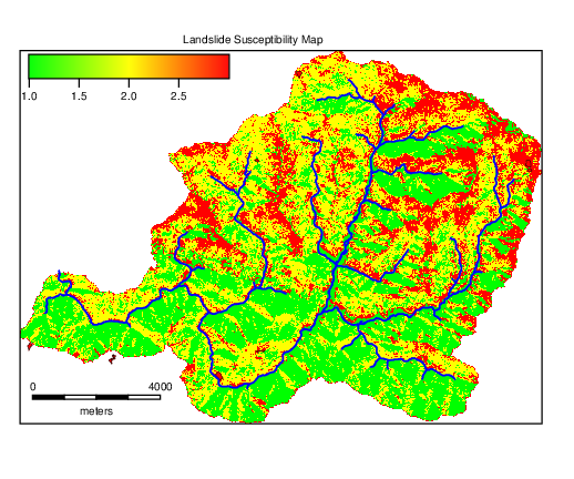
Figure 11.4: Landslide Susceptibility Map