10  Supervised Classification Using Grass-GIS

10.1 Overview of the Workflow

This tutorial demonstrates a robust methodology for land use and land cover (LULC) classification using GRASS GIS. The process integrates:

1. Data Pre-processing (Import and Layer Stacking)
2. Unsupervised Exploration (Clustering)
3. Supervised Classification (Training via QGIS/SMAP)
4. Spatial Refinement (Image Segmentation and Smoothing)

10.2 Data Acquisition via openEO

We will use openEO for data extraction using Copernicus Data Space Ecosystem JupyterLab.

10.2.1 Why use openEO for this workflow?

Using the code from the CDSE samples provides three major advantages:

• Server-side Filtering: Only the requested bands and area of interest (AOI) are processed, saving bandwidth and storage.
• Consistency: The SENTINEL2_L2A collection ensures data is already atmospherically corrected (Bottom of Atmosphere reflectance).
• Reproducibility: The temporal_extent and spatial_extent parameters clearly document exactly what data was used for the classification.

10.2.2 Cloud-based Data Cube Extraction

Accessing Sentinel-2 data directly through the Copernicus Data Space Ecosystem (CDSE) JupyterLab environment using the openeo library allows for efficient filtering and downloading without local pre-processing.

Following Python Source implementation was adapted from Copernicus Data Space Ecosystem (CDSE) sample notebooks and openEO documentation (ESA, 2024). (European Space Agency 2024)

10.2.3 openEO Basics: How to load a data cube from a data collection?

This section provides a detailed guide on how to load a DataCube from a data collection. Additionally, it will cover how to authenticate in order to process and download data.

10.2.3.1 Setup

Import the openeo package and connect to the Copernicus Data Space Ecosystem openEO back-end.

import openeo

## Connect & Authenticate
connection = openeo.connect(url="openeo.dataspace.copernicus.eu")
connection.authenticate_oidc()

10.2.3.2 Supply the Parameters for Data Extraction

s2_cube = connection.load_collection(
    "SENTINEL2_L2A",
    temporal_extent=("2026-01-15", "2026-01-23"),
    spatial_extent={
        "west": 85.79,
        "south": 27.018,
        "east": 86.081,
        "north": 27.329,
        "crs": "EPSG:4326",
    },
    bands=["B02", "B03", "B04", "B08", "B11", "B12"],
    max_cloud_cover=10,
)

10.2.3.3 Download the data cube

s2_cube.download("sentinel_stack") # Change the name of file as necessary

Now you can download the data to your own PC.

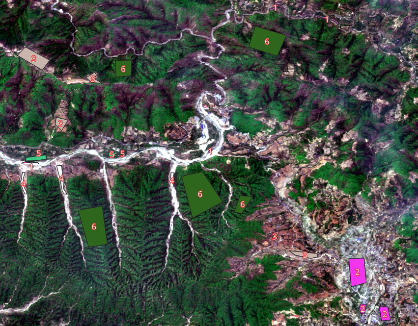
10.3 Prepare Training Dataset in QGIS

• Create polygon layer with an land-use id field
• Create polygons with different land uses (e.g. forest, barren land, built-up area, water-body etc.)

Sample Landuse Training Data

10.4 Environment Setup and Data Import

The workflow begins by importing the multispectral Sentinel-2 imagery and the training vector data prepared in QGIS.

# Import the multispectral raster stack
r.import input=kamalamai.tif output=kamalamai

# Import training polygons (Geopackage)
v.import input=rs_practice.gpkg layer=lu_train output=lu_train

!(import-screenshot.png)

10.5 Displaying the image as RGB

i.colors.enhance red=redband green=greenband blue=blueband strength=90

d.rgb red=redband green=greenband blue=blueband

10.6 Spectral Indices and Feature Enhancement

To improve classification accuracy, additional bands like NDVI (Normalized Difference Vegetation Index) are generated. This highlights chlorophyll content and separates vegetation from bare soil.

# Generate NDVI from Red (Band 3) and NIR (Band 4)
i.vi output=ndvi.B2_12 viname=ndvi \
     red=B2_8_B11_12.3 nir=B2_8_B11_12.4

!(ndvi-map.png)

10.7 Supervised Classification Strategy

Supervised classification requires converting vector training sites into a raster format that the GRASS engine can process.

10.7.1 Step A: Rasterizing Training Data

v.to.rast input=lu_train output=train_data \
          use=attr attribute_column=lu_id

10.7.2 Create Group and Subgroup

i.group
i.group group=rapti subgroup=subgr_B2_12.rapti input=rapti.B2,rapti.B3,rapti.B4,rapti.B8,rapti.B11,rapti.B12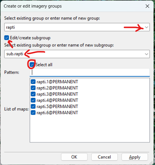

Run i.group

10.7.3 Step B: Signature Generation

The i.gensigset command calculates the spectral statistics for each class ID.

i.gensigset trainingmap=train_data group=B2_8_B11_12 \
            subgroup=subgr_B2_12 signaturefile=supervised.sig

10.8 SMAP Classifier

We will SMAP Classifier in GRASS GIS. In the context of GRASS GIS and image processing, Sequential Maximum A Posteriori (SMAP) is a sophisticated supervised classification algorithm that goes beyond standard pixel-by-pixel analysis.

While common classifiers like Maximum Likelihood (ML) treat each pixel as an isolated data point, SMAP considers the spatial context—the relationship between a pixel and its neighbors—to produce a cleaner, more accurate map.

10.8.1 How SMAP Works

The core logic of SMAP (Bouman and Shapiro 1994) is built on Bayesian Statistics. In simple terms, it calculates the “posterior probability” (the probability that a pixel belongs to a class given its spectral data) by combining two things:

1. Likelihood: The spectral information from the image bands.
2. Prior Probability: Information about the spatial structure of the landscape.

The “Sequential” part refers to a Multiscale Random Field (MSRF) approach. The algorithm looks at the image at multiple scales (from coarse to fine):

• It first classifies larger blocks of pixels.
• It then refines these classifications at finer scales, ensuring that a pixel’s class is consistent with the general land cover of its surrounding region.
• This effectively filters out “spectral noise” (the salt-and-pepper effect) without losing significant spatial detail.

10.8.2 Comparison: ML vs. SMAP

Feature	Maximum Likelihood (ML)	SMAP
Logic	Pixel-by-pixel	Regional/Contextual
Noise Handling	High (produces “salt and pepper”)	Low (smooth, contiguous regions)
Computational Complexity	Simple/Fast	Complex/Slower
Accuracy	Good for spectral outliers	Superior for homogeneous areas

This methodology is particularly favored for Sentinel-2 and Landsat data because it mimics how a human interpreter looks at a map—recognizing that a single “forest” pixel is more likely to exist inside a forest patch than in the middle of a lake.

10.9 Executing the SMAP Classifier

The SMAP (Sequential Maximum A Posteriori) classifier is used because it considers the spatial context of pixels, reducing the “salt and pepper” noise common in traditional Maximum Likelihood classifications.

i.smap group=B2_8_B11_12 subgroup=subgr_B2_12 \
       signaturefile=supervised.sig output=supervised.class

10.10 Post-Processing: Object-Based Smoothing

Raw pixel-based results often contain isolated misclassified pixels. A segmentation-based smoothing approach creates a more professional “map-like” appearance.

1. Segmentation: Groups pixels into homogeneous objects.
2. Mode Filtering: Assigns each segment the most frequent class found within its boundary.

# Step 1: Segmentation
i.segment group=seg_group output=segments threshold=0.4 minsize=20

# Step 2: Smoothing using the 'Mode'
r.mode base=supervised.class cover=segments output=classified_smoothed

10.11 Statistical Analysis and Export

The final step involves quantifying the area of each land use category and exporting the result for use in external GIS software.

10.11.1 Reporting Areas

r.report map=classified_smoothed units=h,p

10.11.2 Exporting to GeoTIFF

r.out.gdal input=classified_smoothed \
           output=final_lu_classification.tif format=GTiff

!(final-map.png)

10.12 Summary Table of Commands

Phase	GRASS Tool	Purpose
Import	r.import / v.import	Loading data into the database
Indices	i.vi	Calculating NDVI
Training	i.gensigset	Extracting spectral signatures
Classify	i.smap	Contextual supervised classification
Refine	i.segment + r.mode	Smoothing and noise reduction

A detailed breakdown of the i.segment threshold is essential because the parameter directly controls the “granularity” of the objects created. In the context of Sentinel-2 data, which typically has resolutions of 10m (Visible/NIR) and 20m (Red Edge/SWIR), the threshold determines whether small features like individual buildings or narrow roads are preserved or merged into the surrounding landscape.

10.13 Understanding the Segment Threshold

The threshold parameter in GRASS GIS ranges from 0.0 to 1.0. It represents the spectral “distance” allowed between pixels to be considered part of the same segment.

10.13.1 Threshold Settings for Sentinel-2

Threshold Value	Resulting Object Size	Best Use Case
0.01 - 0.1	Very Small (Over-segmentation)	Detecting small urban structures or narrow drainage lines in 10m bands.
0.2 - 0.4	Balanced Objects	General LULC (Forest patches, agricultural fields, water bodies).
0.5 - 0.7	Large (Under-segmentation)	Broad regional mapping where local variance (e.g., individual trees in a forest) should be ignored.

10.14 Parameter Selection by Resolution

Since Sentinel-2 bands have different spatial resolutions, the i.segment behavior changes based on the group composition.

10.14.1 10m High-Resolution Bands (B2, B3, B4, B8)

At 10m resolution, spectral variance is high. A lower threshold (0.1 to 0.25) is often required to prevent the “bleeding” of urban edges into vegetation.

10.14.2 20m Mid-Resolution Bands (B5, B6, B7, B11, B12)

These bands provide better chemical/moisture differentiation but lose spatial detail. When using these, a slightly higher threshold (0.3 to 0.45) is effective for capturing homogeneous agricultural blocks or large wetland areas.

10.15 Interaction with minsize

The minsize parameter acts as a secondary filter. It ensures that no segment is smaller than a specific number of pixels, regardless of the threshold.

• For 10m Data: A minsize=10 ensures features are at least 1,000 \(m^2\).
• For 20m Data: A minsize=10 ensures features are at least 4,000 \(m^2\).

10.15.1 Optimal Combined Strategy

To achieve the smoothing seen in the previous tutorial steps, the following parameters are recommended for standard Sentinel-2 LULC (Grippa et al. 2017):

# Optimized for 10m/20m fused stacks
i.segment group=seg_group \
          output=segments \
          threshold=0.3 \
          minsize=15 \
          memory=2000

10.16 Impact on Post-Classification Smoothing

When r.mode is applied using these segments, the choice of threshold dictates the “smoothness” of the final map:

• Low Threshold: Keeps the map detailed but may retain some classification errors.
• High Threshold: Results in a very clean, vector-like map but may eliminate small, legitimate land-use classes (like isolated farmhouses or small ponds).

10.17 Sensitivity Analysis

Performing a Sensitivity Analysis allows for the identification of the “sweet spot” where the threshold is high enough to remove noise but low enough to preserve significant land-cover boundaries. In GRASS GIS, this is best achieved using a simple loop script (Bash or Python) to generate multiple iterations for comparison.

10.17.1 Automated Threshold Iteration

To evaluate the impact of the threshold, a series of segmentations is run across a range of values (e.g., 0.1 to 0.5).

# Example Bash loop to test thresholds 0.1, 0.2, 0.3, 0.4, 0.5
for t in 0.1 0.2 0.3 0.4 0.5; do
    i.segment group=seg_group output=seg_t_$t threshold=$t minsize=20 --overwrite
done

!

10.17.2 Mathematical Evaluation Metrics

Visual inspection is subjective. To determine the “optimal” value mathematically, two primary metrics are often calculated:

10.17.2.1 A. Intra-segment Variance (Weighted Variance)

This measures how “pure” the segments are. As the threshold increases, segments become larger and more heterogeneous, causing the variance within each segment to rise.

10.17.2.2 B. Inter-segment Heterogeneity (Moran’s I)

This measures the contrast between neighboring segments. An optimal segmentation should maximize the difference between a segment and its neighbors while minimizing the internal variance.

10.17.3 The “Elbow Method” for Optimization

By plotting the Weighted Variance against the Threshold, an “elbow” or a point of diminishing returns is usually visible.

1. Low Thresholds: Low variance but too many segments (over-segmentation).
2. High Thresholds: High variance and loss of detail (under-segmentation).
3. Optimal Point: The value just before the variance begins to spike sharply.

10.17.4 Implementation Workflow in GRASS

To find this optimal value without manual calculation, the following workflow is applied:

10.17.4.1 Step 1: Calculate Variance for each Threshold

After running the loop in Section 1, use r.univar to check the variance of the original imagery within the generated segments.

# Check variance of the NIR band (B8) within the segments
r.stats.zonal base=seg_t_0.3 cover=B2_8_B11_12.4 method=variance output=var_t_0.3
r.univar map=var_t_0.3

10.17.4.2 Step 2: Compare Results

Threshold	Segment Count	Mean Internal Variance	Observation
0.1	15,400	12.5	Over-segmented; retains noise.
0.3	4,200	18.2	Potential Elbow; clean boundaries.
0.5	850	54.8	Under-segmented; forest and urban merged.

10.17.5 Selection for Supervised Classification

Once the optimal threshold is identified (e.g., 0.3), that specific segment map is used as the base for the final r.mode smoothing of the i.smap output.

# Using the mathematically optimal segments to smooth the classification
r.mode base=supervised.class cover=seg_t_0.3 output=final_refined_classification

10.18 Assessment of Accuracy

To evaluate the reliability of the classification, a statistical comparison between the classified map and independent reference data is required. This process typically utilizes a Confusion Matrix (also known as an Error Matrix), which generates the Kappa Coefficient and Overall Accuracy.

10.18.1 Preparation of Validation Data

Accuracy assessment requires a set of reference points that were not used during the training phase. If a separate validation dataset does not exist, the original training vector can be split into two subsets: one for training and one for validation.

10.18.2 Create Random Validation Points

If ground truth polygons exist, random points can be generated within them to act as validation sites.

# Generate 50 random points per class from the validation vector
v.random.cover input=validation_vector output=val_points npoints=50 column=lu_id

10.18.3 Generating the Confusion Matrix

In GRASS GIS, the r.kappa module compares two raster maps: the Classification Result and the Reference Raster (the rasterized validation points).

10.18.3.1 Step A: Rasterize Validation Points

v.to.rast input=val_points output=val_points_rast use=attr attribute_column=lu_id

10.18.3.2 Step B: Run Accuracy Analysis

r.kappa classification=final_refined_classification \
        reference=val_points_rast \
        output=accuracy_report.txt

10.18.4 Interpreting the Results

The output file (accuracy_report.txt) provides several critical metrics:

10.18.4.1 A. Overall Accuracy

The simplest measure, calculated as the total number of correctly classified pixels divided by the total number of reference pixels.

10.18.4.2 B. Producer’s Accuracy (Omission Error)

Measures how well a specific real-world land cover type was classified. If 80 out of 100 actual forest pixels are correctly identified, the Producer’s Accuracy is 80%. The remaining 20% is the Omission Error.

10.18.4.3 C. User’s Accuracy (Commission Error)

Measures the reliability of the map for the user. If the map says a pixel is “Urban,” how often is it actually “Urban” on the ground? If the map shows 100 urban pixels, but only 70 are correct, the User’s Accuracy is 70%. The remaining 30% is the Commission Error.

10.18.5 The Kappa Coefficient ()

The Kappa coefficient is a more robust metric because it accounts for the possibility of the classification occurring by random chance.

Kappa Value	Strength of Agreement
< 0.40	Poor to Fair
0.40 - 0.60	Moderate
0.60 - 0.80	Substantial
> 0.80	Almost Perfect

10.18.6 Iterative Improvement

If the accuracy for a specific class (e.g., “Water”) is low, the workflow should return to the Signature Generation or Segmentation phase:

1. Check Training Data: Ensure training polygons are spectrally “pure.”
2. Adjust Threshold: If urban and bare soil are confused, the segmentation threshold might be too high, merging distinct spectral signatures.

10.19 Summary of Accuracy Workflow

Step	Command	Goal
1	v.random	Create independent validation sites
2	v.to.rast	Prepare reference data for comparison
3	r.kappa	Calculate Matrix and Kappa statistics
4	r.report	Compare area distributions

Bouman, C. A., and M. Shapiro. 1994. “A Multiscale Random Field Model for Bayesian Image Segmentation.” IEEE Transactions on Image Processing 3 (2): 162–77. https://doi.org/10.1109/83.277898.

European Space Agency. 2024. openEO Basics: How to Load a Data Cube from a Data Collection. Copernicus Data Space Ecosystem. https://dataspace.copernicus.eu/.

Grippa, Taïs, Moritz Lennert, Benjamin Beaumont, Sabine Vanhuysse, Nathalie Stephenne, and Eléonore Wolff. 2017. “An Open-Source Semi-Automated Processing Chain for Urban Object-Based Classification.” Remote Sensing 9 (4). https://doi.org/10.3390/rs9040358.