Chapter 3 Coordinate Reference System
After reading and practicing the first two chapters that you can do everything in GIS or QGIS. But, many things are still to know. We might want to know how QGIS knows where to place a point or a line or a polygon or a raster image. It requires the location of these features. Locations are expressed in terms of coordinates. Now is the time to upgrade yourself and learn a few things about coordinate reference system. We might be able to display maps without the knowledge of coordinates, but for analysis and understanding of GIS data we need to know how the locations are conceived in GIS.
3.1 What is coordinate
Most of us might have the concept of coordinate which we studied in school. However, they only deal with points in plane. Let us recollect what we learned earlier. Points in the plane can be simply plotted with their coordinates as shown in figure 3.1

Figure 3.1: Concept of coordinate
As the earth is not plane but curved, we need to learn a bit about the shape of earth and its geometry. Shape of the earth can be fairly assumed to be a sphere. Let us think about a line (axis) passing through the north pole and south pole. We can draw a circle surrounding the earth passing exactly at the centre of this axis. This is called equator. We can draw circles parallel to the equator such that they subtend a given angle at the equator. Figure 3.2 shows the earth, the axis, equator and the circles parallel to the equator. The angles formed at the equator is shown in degrees. This angle is called latitude.

Figure 3.2: Concept of Latitude
Now, we understand one part of the coordinates. We can draw lines from north pole to south pole. Such lines will be a half circle. These are called meridians. The meridian passing through Greenwich, London of United Kingdom is considered as the reference meridian and is also known as prime meridian. Locations East of the meridian are taken as positive and towards west are taken as negative, see figure 3.3.
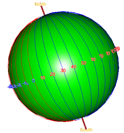
Figure 3.3: Concept of Longitude
The frame (above) shows a movable and zoomable 3D image of sphere with latitude and longitude. Somewhere on the sphere you can see a map of Nepal. It is made with \(R\) programming language. By draging with mouse or moving the mouse wheel the image can be rotated and zoomed. You can see that Nepal is situated between around \(26~to~30^\circ\) latitude and \(80~to~90^\circ\) longitude. Any point on the earth can be, now, expressed in terms of latitude and longitude. As we can see, the latitude varies from \(-90^\circ\) to \(90^\circ\). The negative value represents locations south from the equator and positive means north of equator. Similarly, longitude varies from \(-180^\circ\) to \(180^\circ\). Negative value represents locations west from the prime meridian and positive means east of prime meridian. A point on earth can be reprsented for example as (85.5732, -27.3456) or (85.5732E, 27.3456S). ‘E’, ‘W’, ‘N’, ‘S’ is, obviously, short form for the four directions. Try the following exercise.
- Open https://www.google.com/maps.
- In the search box type ‘27.7, 85.312’ (without quotes) and click enter.
You will find the map centered at the point (85.312E, 27.7N). Google maps uses latitude first.
We have shown the latitudes and longitudes on sphere in the above images. You might think that your knowledge of coordinates is complete with this information. However, in GIS we don’t work with 3-dimensional display. You might recall the map of the world we created in the first exercise 1.4.1. When you display the map in cartesian coordinates, the map stretches from -180 to 180 degress in x-direction and -90 to 90 degrees in y-direction. However, if you check the sphere above, you can see that -180 degrees (180 degrees west) and 180 degrees (180 degrees east) represents the same line. Simiarly, we can see that the circles parallel to the equatorial one get smaller as we go towards north or south. However, on the flat display, it is not the same. The distance between places get highly exaggerated as we go farther from equator. These and few more things, make it essential to devise better ways to represent the locations more accurately on the plane map. In simple words, we can say that ‘it is impossible to reprsent any part of earth accurately on a two dimensional plane’. Only a three dimensional globe can represent the locations close to the actual. Many approaches has been devised and in practice to minimize the loss of accuracy. We will try to understance some of them in the following sections.
3.2 Projection and projected coordinate system
In the first exercise 1.4.1, we used latitude and longitude as x-coordinate and y-coordintae respectively. This is called *geographical coordinate system** (GCS).
We can not put whole the globe on a plane paper. However, we can represent a small portion of globe with higher accuracy. The methods of representing curved surface of globe on a plane surface is called projection. Let us think how we can do this.
3.2.1 Transverse Mercator Projection
We can put a sphere inside a cylidnder of the same (almost) diameter. One of the big circles of the sphere will touch the inside of cylinder. You can imagine this with the help of following frame. This, again, can rotated zoomed etc.
As we can see, a thin strip of the cylinder almost touches the surface of globe. We can project this small strip of the globe on the cylinder. And, cylinder can be unfolded to make a plane surface. Thus we can achieve our aim of representing a part of globe on plane paper.
In the above frame, the cylinder is placed horizontally (if we consider north-south as vertical) so that a meridian coincides with the cylinder. If we place the cylinder vertically, in the same sense, the resulting projection is called Mercator Projection. Hence, when tilted \(90^\circ\) it is called ‘Transverse Mercator Projection’.
3.2.1.1 Universal Transverse Mercator (UTM) Projection
We can see in the same frame, that the globe is divided into \(6^\circ\) angles and the cylinder touches the meridian passing through \(3^\circ\). In this way, we can project \(0^\circ\) to \(6^\circ\) on the cylinder. This is a universally accepted division of globe into 60 strips at \(6^\circ\) intervals starting from \(-180^\circ\) (\(180^\circ~W\)) to \(180^\circ\)(\(180^\circ~E\)). This projection system is called ‘Universal Transverse Mercator Projection’. It is denoted as a number with ‘N’ or ‘S’ where the number reprsents the strip count from \(180^\circ~W\). For example, the strip passing from longitude \(180^\circ~W\) to \(174^\circ~W\) will be denoted as ‘1N’ if it is in northern hemisphere. If you calculate using the same method, you can find that Nepal which stretches from around \(80^\circ~E\) to \(90^o~E\) must use two different projections for two halves of the country. Projection ‘44N’ will be used for the area lying west of \(84^\circ~E\) (\(78^\circ~E\) to \(84^\circ~E\)) and ‘45N’ will be used for the area lying east of \(84^\circ~E\) (\(84^\circ~E\) to \(90^\circ~E\)).
3.2.2 Azimuthal Projection
Another way of projecting the globe is using a plane. This is called Azimuthal Projection. In the following frame, the concept of Azimuthal Projection is made clear.
In the above figure, we can observe two things: 1) Azimuthal projection can show half of the globe at most, 2) The distance between latitude circles become smaller as go to the equator.
Second point can be corrected by expanding the circles such that the distance between consecutive latitudes are equal. As such, there are several ways we can use azimuthal projection. However, we will not go into detail as it will get more complex.
3.2.3 Conic projection
As the name suggests, we may put the globe inside a cone, so that a portion of cone almost coincides with the globe. Check the following frame. Similar to a cylinder, a cone can also be flattened. This is the concept of Conic projection.
3.2.4 Summing up the projection
We explained three types of chiefly used projections briefly, in fact, very briefly. You may go into depth by looking for ‘Cartography Projection’ or something similar on an internet search engine. One of the result I have found is http://www.progonos.com/furuti/MapProj/Normal/CartHow/cartHow.html. Here, you can find a lot of informative materials about these projections.
So, what are the three projections? They are:
Cylindrical projection : Transverse mercator projection is one kind of cylindrical projection. UTM (Universal Transverse Mercator) projection is again the Transverse mercator projection for the zones of different part of the globe.
Azimuthal projection
Conic projection
Selecting a proper projection system depends on the accuracy provided by it. Which is in turn governed by the location of the place on the globe. Every countries in the world have standardised the use of the projection system. In Nepal, we use two UTM projections 1) UTM 44N and 2) UTM 45N. We don’t use conic or azimuthal projection.
3.3 Shape of earth
Generally, we would find the explanation about the shape of earth before the projection system in most of the books. However, I ended up opposite. Anyway, let us briefly touch this subject.
So, what is the shape of earth? We see a lot of mountains, undulations etc on the earth. Do they count in the shape of earth? Actually, we are supposed to draw a surface of same elevation over whole the earth and it should pass through the surface of sea. It may be easy for some. To make such surface you will have to cut the Everest and fill the Dead Sea up to the zero-level. Now you might have some idea.
When we draw a surface passing at zero elevation, we will get somewhat ellipsoidal surface. It is not spherical. The shape can be created by making an ellipse and revolving around y-axis. Still, the shape is not exactly an ellipsoid. However, for most practical purposes we take it to be an ellipsoid. Some of the properties of this ellipsoid are mentioned below:
Diameter passing from North pole to South pole is less than the diameter at equator. See Figure 3.4.
The shape of earth is defined by the diameter at equator and flattening ratio. If we consider the radii of ellipse as shown in the figure, the flattening ratio will be given by \((a-b)/a\).
There are many approximations of the shape of earth which are in use world wide. Each of such approximate assumed shape of earth is given a name and called Datum.
Most commonly used Datum is known as WGS84. The flattening ratio for WGS84 is around \(1/298\). The radius at equator is 6378137 meters.
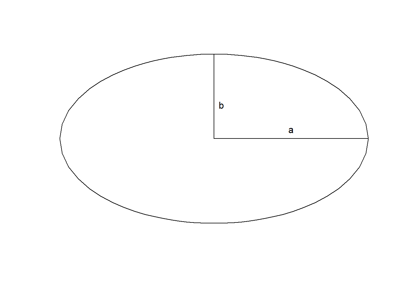
Figure 3.4: Shape of earth and its parameters
Datum (the assumed shape of earth) and the projection in combination is used to define a Coordinate Reference System. Following combinations and many more are possible:
- WGS84 (datum) and Geographic coordinate system (Without projection)
- WGS84 and UTM 45N (It can represent only \(84^\circ\) to \(90^\circ\) East only)
- JGD2000 and Geographic coordinate system
- JGD2000 and UTM 53N (some portion of Japan)
We will try to understand some details with exercise.
3.4 Projection Transformation
Let us recall the first exercise where we displayed the world countries. We had used ne_50m_admin_0_countries shapefile to display data. Let us have a look at the data. Browse the folder Exercise01 using windows file explorer. You can see multiple file with the same name but different extensions as:
- ne_50m_admin_0_countries.shp
- ne_50m_admin_0_countries.dbf
- ne_50m_admin_0_countries.prj
- ne_50m_admin_0_countries.shx etc.
These files as a set make up a shapefile which is one of the formats of GIS vector data. You may not be able to display the data in GIS if any of the files is missing. File with extension .prj contains the information about the type of Coordinate Reference System used in the shapefile.
3.4.1 Exercise - 1 (Assigning projection)
We had used some zip files in the second chapter. Let us create a folder Exercise03 and unzip the admin-palika.zip and 1000k.zip.
Let us have a look inside the unzipped folder.
For example, there is a shapefile named admin_ar inside 1000k. The file with extension .prj is missing. Which means that this shapefile does not have projection information. Let us try to display it in QGIS. What happens?
You will see a warning message ‘CRS was undefined, defaulting to EPSG:4326 WGS84’. This is because the projection for the shape file is not defined. It is good that QGIS tries to display the data in default CRS, that is, WGS 84 Geographic Coordinate system. Now let us do the exercise in steps:
- Create a folder WGS84 under Exercise03.
- In QGIS we have displayed admin_ar.
- In the list panel right click the layer and click Save as.
Refer to figure 3.5 and follow the next steps. Number in the brackets correspond to the number in the figure.
- In Save vector layer as dialog, click browse (1) and select file name admin_ar_wgs.shp inside newly created WGS84 folder.
- Click the pictorial button (2) for selecting the CRS.
- Coordinate Reference System Selector dialog will be displayed.
Let us observe the dialog. It has six parts. 1) information about the dialog, 2) Filter, 3) Recently used coordinate reference system (it will be empty at first), 4) Coordinate systems of the world 5) Selected coordinate system and 6) detail of the projection. You can explore the coordinate systems of the world by expanding each one.
- In the filter write wgs 84 (3). Matching names will be displayed in the list inside Coordinate systems of the world.
- Select WGS 84 (4) under Geographic Coordinate system and click OK (5).
- Click OK in the Save vector layer as dialog.
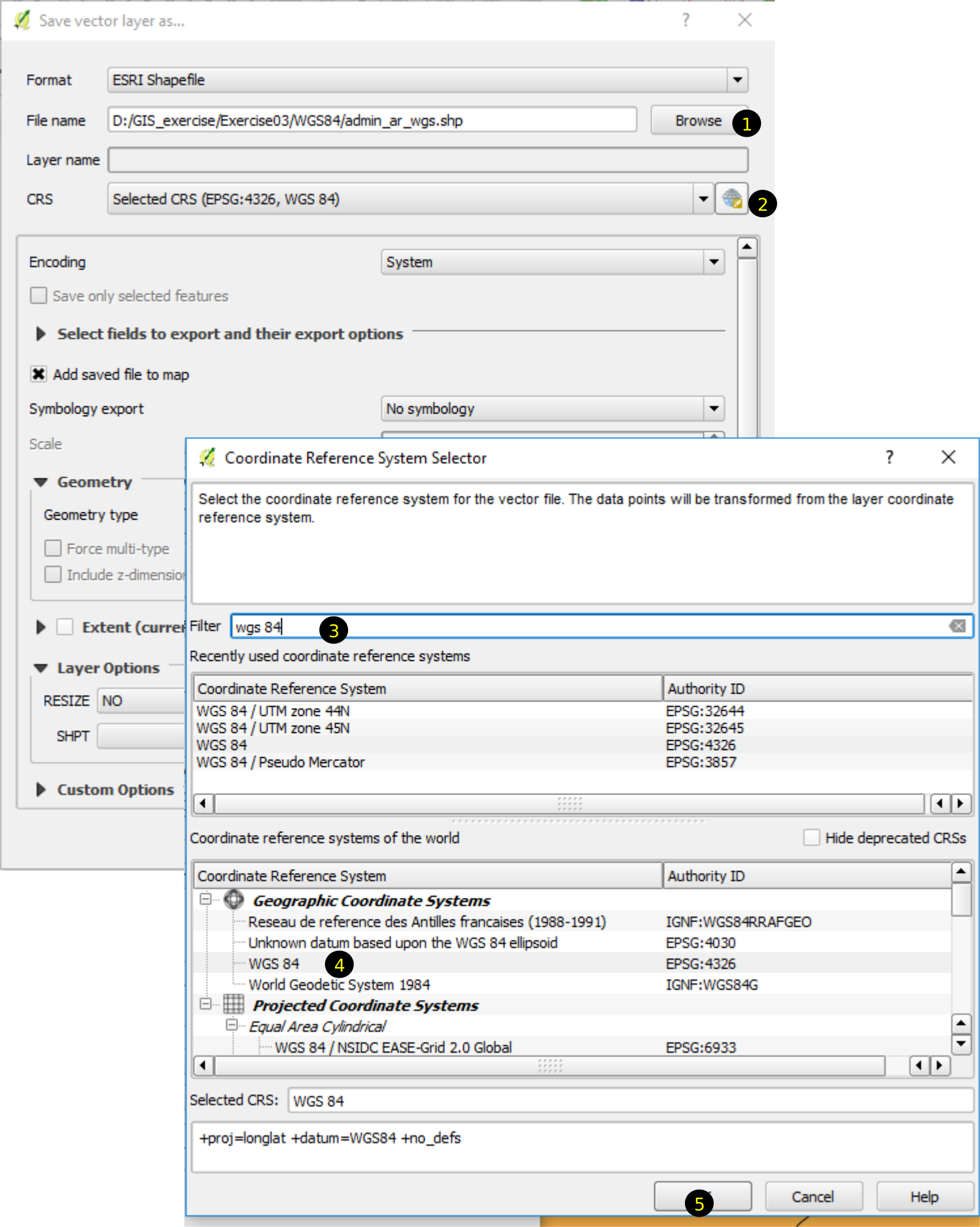
Figure 3.5: Assignment or transformation of projection
Let us see the contents of the shapefile inside WGS84 folder. You will see a file with extension .prj. Zoom the map to the extent of admin_ar layer. Move the cursor on the map and observe the coordinates in the status bar. The x-coordinates will be \(80\) to \(90\) and y-coordinate will be \(25\) to \(30\).
Repeat the above exercise for other shapefiles, for example, admin_ln in the directory 1000k. Let us compare the projection (.prj) files created for each shapefile. You can open these projection files with Notebook or any text editing software. By examining the two files you can see that they are completely identical. Which means you can:
- copy admin_ar_wgs.prj which is created in the new directory (WGS84) and
- paste into 1000k directory and change the name of file to admin_ar.prj.
- Now, if you add the admin_ar shapefile in QGIS it will not show any warning.
- In the same way, you can copy-paste the projection file and rename it to match the remaining shapefiles.
3.4.2 Exercise - 2: Projection transformation of vector data
In the above exercise we assigned the projection to the shapefile. In the next exercise, we will transform the shapefile, which is currently in WGS84 Geographic Coordinate system, to another projection. This process is called projection transformation. In the following exercise, we are going to:
- Change the CRS of the shapefile of administrative boundaries of Nepal from User CRS to WGS84
- Select the features of province 1.
- Transform the CRS of the shapefile again to UTM 45N.
Let us follow the steps below :
- User CRS to WGS84
- Create a new folder UTM inside Exercise03
- In QGIS, click New tool from Project toolbar .
- You may save or discard previously opened file.
- Now add the vector layer ADMIN_GAPANAPA inside folder admin-palika to the map. Observe the right corner of the status bar (figure @(fig:statusBarCRS). It shows the CRS of the shapefile. We see a small globe icon and User 100000. This is the CRS of current map. If you hover over the map you can see some details.
- Follow the previous exercise and save this shapefile in WGS84 folder as admin_gapanapa_wgs.
- Select features from province 1
- Once again click New tool from Project toolbar and save or discard previously opened file.
- Add newly created admin_gapanapa_wgs shapefile to the map. Now once again observe the CRS (right corner of the status bar). Now it is EPSG:4326, which means WGS84 and Geographic Coordinate system.
- From the Attributes toolbar click Select features using an expression tool. This tool has an image of \(\epsilon\).
- In the Select by expression dialog, write expression as
python gpx, python.reticulate=FALSE, eval=FALSE province" = 1. - Click Select at the bottom of the dialog. Close the dialog. You can observe that the features in the province 1 will turn yellow.
- By moving the cursor in horizontal direction above the selected features, you can observe that the coordinates vary from around \(86^\circ\) to \(88^\circ\). Which means the features lie in UTM 45N zone.
- Transform from WGS84 to UTM 45N
- Write click the layer and click Save as.
- In the Save vector layer as dialog, click Browse and save the file as province_1_utm45n inside UTM folder.
- Check Save only selected features in the dialog.
- Click CRS button, CRS selection dialog will appear.
- In the filter write 45n. From the matching CRS in the list, select WGS 84/UTM zone 45n.
- Click OK in the CRS selector dialog and then in the Save Vector layer dialog.
- Click New tool from Project toolbar. Save or discard the current project.
- Add newly created province_1_utm45n shapefile. Once again observe the CRS. It is now EPSG:32645 which means UTM 45N projection. you may save the project as ‘ex03a.qgs’

Figure 3.6: Status bar and CRS(Coordinate Reference System)
3.4.3 What is EPSG?
We saw in the last section that CRS is represented in the form EPSG:n, where n is a number. So, what is EPSG? It is short form of ‘European Petroleum Survey Group’. There are many CRS’s in use and EPSG coded all (most of) the CRS and gave a code to each. Hence, the CRS can be expressed as EPSG:n where n is the EPSG code.
Some EPSG codes and there are name are given below:
- EPSG:4326 WGS84 (World Geodesic System 1984) Geographic coordinate system
- EPSG:32644 Project coordinate system at zone UTM 44N based on WGS84 datum
- EPSG:32645 Project coordinate system at zone UTM 45N based on WGS84 datum
http://spatialreference.org/ is the best place to find different spatial references (Coordinate reference system), their meaning, locations and codes. You are advised to spend at least an hour or two to acquaint yourself to the meaning of CRS.
3.4.4 Projection transformation of raster data
From above examples, we understood that the GIS software can transform vector data from one CRS to another CRS in simple steps. What is involved in transforming vector data? Basic element of a vector data are points. Lines and polygons are formed by joining points. We need to find the coordinates of each point (with known coordinates in one CRS) in new CRS. It is done by using simple formula. We don’t need to know the formula of transformation as it is done by QGIS internally. Theory behind the process of transforming raster data from one CRS to another is a bit complicated compared to the transforming of vector data. Observe figure 3.7. It shows a rectangular grid created in WGS84(GCS) on the left and the same when viewed in WGS84(UTM45N). We can see that the lines are curved and tappering. We know that the raster data are made of rectangular cells. Therefore, simple transformation of each grid cells cannot produce the new raster. As such, in principle, we need to create a raster of same size with selected cell size in new CRS and then copy the values from corresponding cells in the original raster data. This process is called warping. The process may sound complecated but GIS accomplishes the task without any difficulty. We will show this in the following exercise.
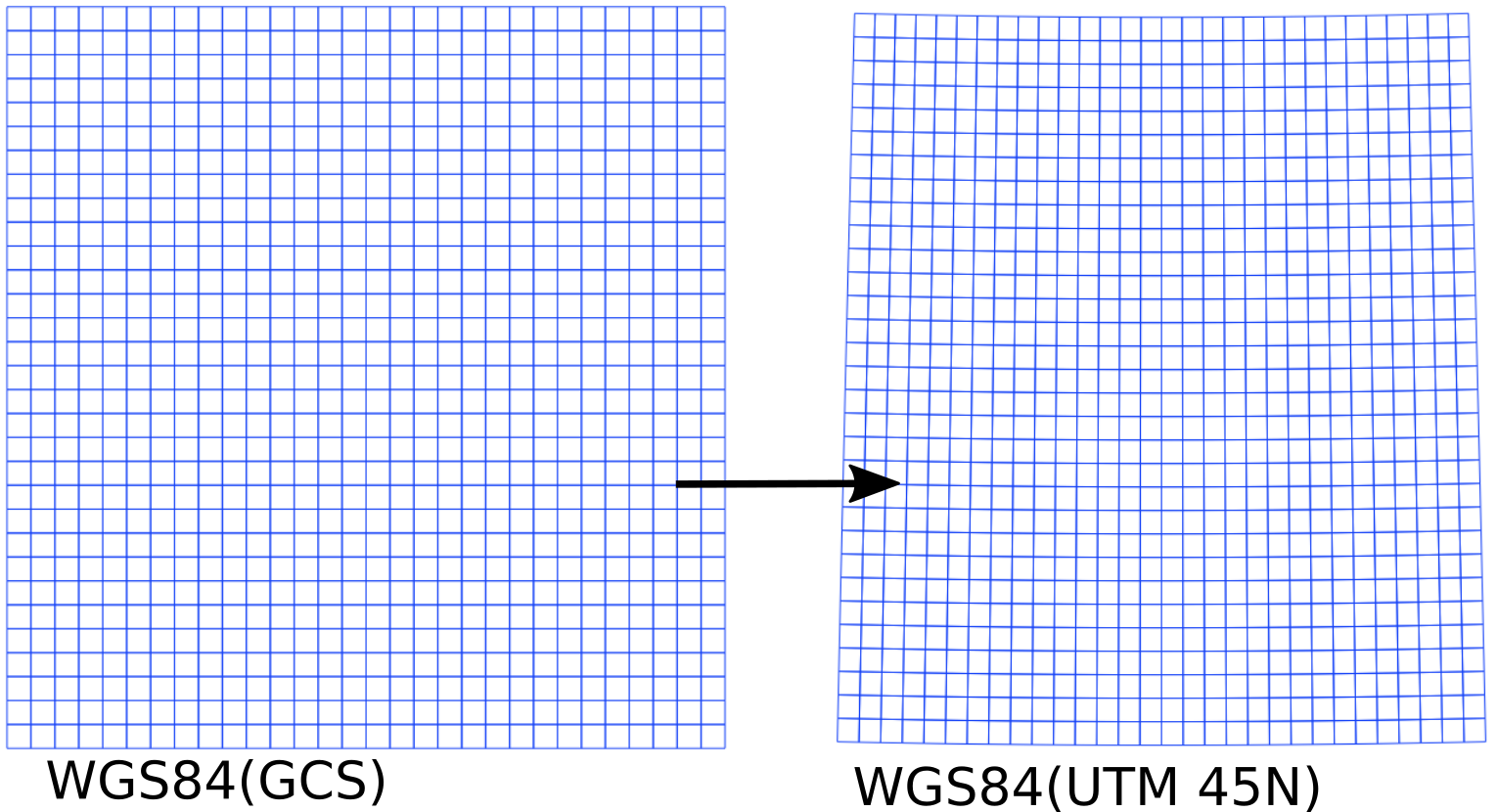
Figure 3.7: Rectangular grid in two different CRS
3.4.5 Exercise-3: Projection transformation of raster data, step by step
We will use the elevation data which we used in Chapter 2. Follow the steps below.
- Add raster data (ASTGTM2_N27E086_dem.tif) to the map.
- Let us observe the data. The CRS is EPSG:4326 which means it is WGS84(GCS). Write click the layer and click Properties.
- Select Metadata in the dialog box, left pane. You can see various properties associated with the data. (Note: all GIS data has associated metadata which gives you many important information).
- Scroll down the right pane to view the properties section which has its own vertical scroll bar.
- Scroll down this section to find various properties such as Statistics, Dimensions, Pixel Size, Extent etc.
- You can see that size of each pixel is around \(0.000278^\circ\). The extent of the data is from around 86 to 87 in x-direction and 27 to 28 in y-direction.
- If we need to change the data to UTM projection, we need to select the UTM zone. From the data, it is clear that it lies in UTM 45N zone.
- From menu, click \(Raster \Rightarrow Projections \Rightarrow warp(Reproject)\). In the next steps the numbers in brackets are associated with the numbers in the figure 3.8.
- Select Output file (1) and save the output in the UTM folder.
- Check Target CRS (2). Select CRS by writing 45N in the filter and selecting EPSG:32645 from the list (3).
- Set the resampling method as Near(4).
- Set No data values as -9999 (5).
- Click OK (6). In the confirmation dialogs click OK and finally click Close on Warp(reprojection) dialog. You may save the project as ‘ex03b.qgs’.
- Click New tool from the Projection toolbar. Add the newly created raster elevation data to the map. You can observe the corners by zooming. You can also find the cell size of the newly created raster data. How?
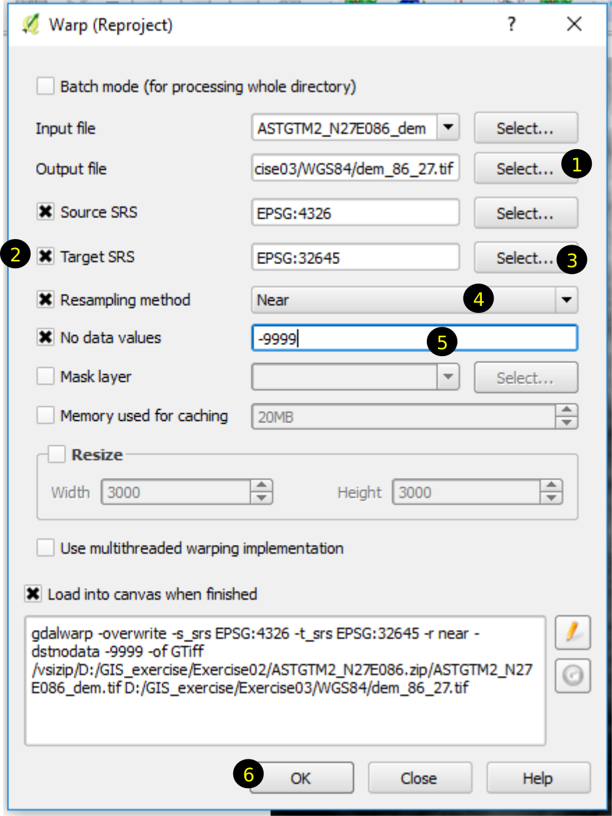
Figure 3.8: Transformation of raster data from WGS84(GCS) to WGS84(UTM45N)
3.5 Why do we need so many different CRS?
When you tried to select CRS in the last exercises, you might have observed that there are 100s of CRS in use. You might question the necessity of having so many CRS. Some points below, can provide you the reason for this.
- WGS84 is the most used datum worldwide. However, the shape of earth assumed by this datum does not fit well whole the world. As such many countries have developed different models (assumed shape) of the earth which fits the shape of a given portion of the earth. Some examples are:
- JGD2000 : Known as Japan Geodetic Datum, it fits the shape of earth at or near Japan.
- NAD 1983: North American Datum etc
- Geographic coordinate system (GCS) gives the most accurate location of a place. That is why many GIS data are available in GCS. Examples are:
- Google map
- Many satellite data (ASTER DEM elevation data etc)
However, it is difficult to show the data on a flat surface.
Distance, area and other geometric calculations are not possible in GCS.
These are the reasons we need to switch the GIS data from one coordinate system to another. We also need to work in different projections. That is why, it is necessary to know which projection we need to work for a given situation. However, we don’t need to go in depth about the process of transformation and theories behind them. Geodesy, in itself, is a vast subject which needs effort to master. Meanwhile we can do our GIS with the knowledge provided in this chapter.