  rm(list = ls())
  clrs = rainbow(4)
  getwidth <- function (spd){
    if(spd < 5) 6
    else if(spd<50) 4
    else if(spd <20) 2
    else 1
  }
  getcolor <- function(spd){
    if(spd < 5) clrs[1]
    else if(spd<10)  clrs[2]
    else if(spd <20) clrs[3]
    else clrs[4]
}Background
R is one of the most versatile programming language. It is mostly used for statistical analysis. However, availablity of vast range of libraries developed by enthusiasts, it has become a handy tool for many kinds of analyses. In this example I will show you how we can produce a simple map with GPS tracking result overlayed on openstreetmap.
What do you need?
R: As mentioned above you will need R language installed in your computer.
RStudio: It is optional, however, recommended. It works as IDE ( integrated development environment ) for coding in R.
GPS tracker: We will not start with ‘What is GPS?’. Recent smartphones whether android or iOS have GPS hardware which receives signal from satellites and show your location on your device. Whether you use Google maps or any other mapping app, you can see your location while walking in the street or driving. For the purpose we are talking about in this article, we are going to use osmtracker which is available from playstore in android and most probably available with iOS based devices. You can track with osmtracker and save the output to a file which is stored in ‘gpx’ format.
Apart from whatever have been mentioned above, you will also need basic understanding of GIS to proceed.
How to get R and RStudio, and get started
You can search R download with Google to get the link to the most recent version of R. Similarly you can download the recent version of RStudio. If you are new to programming, you need to go through other resources for learning R programming from scratch. If you have experience of coding in another languages, especially numerical programming language like MATLAB, Scilab etc, it will not take long to dive into R. From here, it will be assumed that you have understood the basic terminology for R and Rstudio and no further elobaration will be provided for common terms.
Like many other languages, R has many libraries which can be installed and loaded into the code for performing particular function.
Installing the libraries
Most of the libraries are pre-installed with the installation of R. Installing required libraries, you need to enter the following code into the console.
install.packages(“xxxx”), where ‘xxxx’ is the name of package. For running the current code, you will need rgdal and openStreetMap packages. rgdal package is needed to read and manipulate GIS data.
Following code help you to convert speed to the color and width of lines plotted above the map.
The libraries
Libraries are loaded with the following code.
    library(rgdal)
    library(OpenStreetMap)
    library(ggplot2)
Tracking with OSMTracker
First of all visit somewhere with your smartphone while osmtracker is tracking your location. Save it and transfer to your PC.
GIS data are made up of multiple layers. The file produced by osmtracker also has layers of data. The following code will display the names of layers of data.
    lyrs <- ogrListLayers("osm-track.gpx")
    print(lyrs)
We are going to using ‘track_points’ from above layers. The track point data is extracted into a variable by using ‘readOGR’ function available from rgdal library. You can also check what kind of data are represented by other layers such as ‘waypoints’, ‘route_points’ etc in similar way.
First of all we plot the map of the area of interest (extent of gpx data) by using the function ‘openmap’ from openStreetMap library. Here extent of the map is hardcoded. However, we can retrieve the maximum and minimum values of coordinates from the gpx data file using R code. In this way, whole the process can be run automatically except the modification of name of data file.
    mp <- openmap(c(27.70,85.33),
                  c(27.67,85.37 ),zoom = 15,
                      type = "osm")
    plot(mp)
    bkpoint=readOGR(dsn = "osm-track.gpx",
                    layer = 'track_points')
Complete listing of code
    library(rgdal)
    library(OpenStreetMap)
    library(ggplot2)
    # lyrs <- ogrListLayers("posts/plot-track/osm-track.gpx")
    # print(lyrs)
    rm(list = ls())
    clrs = rainbow(4)
    getwidth <- function (spd){
      if(spd < 5) 6
      else if(spd<50) 4
      else if(spd <20) 2
      else 1
    }

    getcolor <- function(spd){
      if(spd < 5) clrs[1]
      else if(spd<10)  clrs[2]
      else if(spd <20) clrs[3]
      else clrs[4]
    }

    mp <- openmap(c(27.60,85.32),
                  c(27.70,85.57 ),zoom = 15,
                  type = "osm")
    bkpoint=readOGR(dsn = "posts/plot-track/osm-track.gpx",
                    layer = 'track_points')

    bkpt=slot(bkpoint,"coords") #coordinates of each point of track

    bkp=as.data.frame(
      projectMercator(bkpt[,2],bkpt[,1]))

    mplot = OpenStreetMap::autoplot.OpenStreetMap(mp)

    mplot = mplot +
      geom_line(data = bkp,
                 aes(x = x, y = y), # slightly shift the points
                 colour = "black", size =  5) +
      xlab("X-coordinate (m)") + ylab("Y-coordinate (m)")

    # mplot

    bktime=slot(bkpoint,"data")["time"] # time at each point
    n=length(bkp$x)
    # aplot = ggplot() +
    s = 0 #road length
    tm = 0 # time
    spdall =c()
    tmseq = seq(1,n,5)
    for(i in tmseq){
      t1 = strptime(strftime(bktime[i,1]),"%Y-%m-%d %H:%M:%S")
      t2 = strptime(strftime(bktime[i+5,1]),"%Y-%m-%d %H:%M:%S")
      ds = dist(bkp[c(i, (i+5)),])
      dt = as.double(t2-t1)
      tm = tm+dt
      if(ds>0){
        s = s+ds
        spd = 3.6 * ds/dt
        spdall =c(spdall, spd)
        pt_i = bkp[i:i+5,]
        wd = getwidth(spd)
        mplot = mplot +
          geom_line(data = pt_i,
                    aes(x = x, y = y), # slightly shift the points
                    colour = getcolor(spd), size =  2.5)

      }
    }
    mplot = mplot + theme(legend.position = "bottom")
    mplot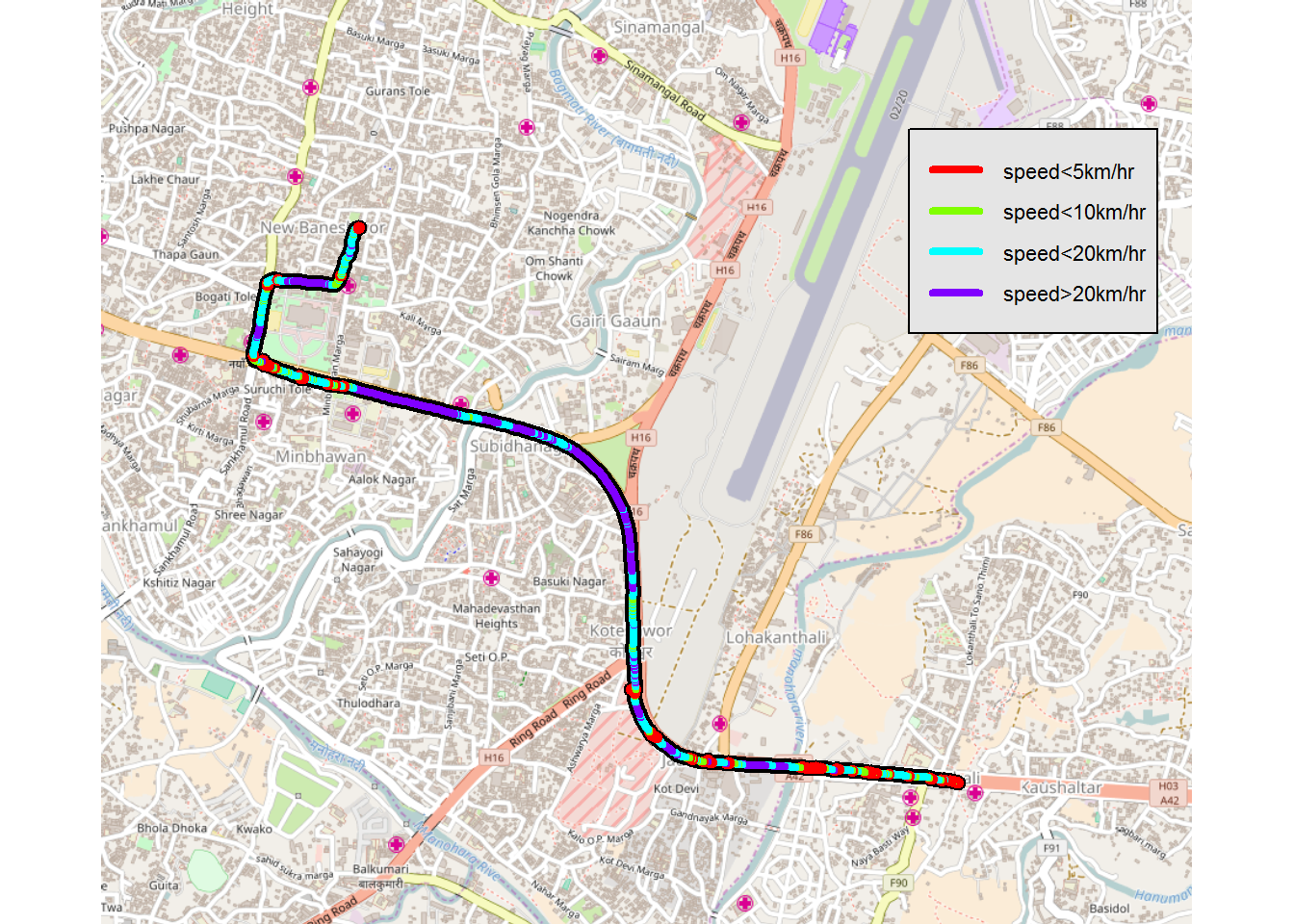
Postscript
In the above code, the ‘track_points’ layer is read into variable ‘bkpoint’. The object ‘bkpoint’ consists of many other objects which can be retrieved by using ‘slot’ function. x and y coordinates of the gps data are stored into ‘coords’. The coordinates need to be transformed into Mercator projection as the openStreetMap does not use geographic coordinate system.
In the follwoing lines of code, we retrieve coordinates of the tracked point and their time. In the following ‘for loop’ we calculate speed for each segment and plot lines in different colors based on the speed. The above code demonstrates the capability of R for plotting a map automatically from observed gpx data. We can automatize map and report production to our need by combining different sources of data.
We can also derive following conclusion from visual interpretation of the map.
Although the speed for maximum length of the stretch seems to be higher than 20km/hr, we can see that it is very slow at some locations. Small stretches where the speed is less than 5km/hr consumes considerable time driving. There are long stretches where speed less than 10km/hr. It took more than 35 minutes to cover 5 km by motorbike which is considered to be the fastest on the Kathmandu roads.
Happy coding!