Preface
Let us learn the practical use of Network Analysis. We will also learn python as used with QGIS. You need very basic understanding of python. A few codes are introduced for practice. Which will help you learn the basics with faster pace. For proper learning of python please refer to other resources.
This tutorial will teach you the followings:
Basics of python
Using QGIS python console and coding interface
Variables, list, tuple, dictionary etc.
Loops (for), if-else statements
Using QGIS python coding interface to
- add-remove layers
- extract vector layer features
- extract feature geometry
- extract feature attribute
Using QGIS python coding to run processing algorithms
Solving GIS problems related to Network analysis
1 QGIS python coding interface
QGIS python console is displayed by using QGIS menu: Plugins\(\Rightarrow\)Python Console or it can simply be opened by using keyboard: Ctrl-Alt-P.
In this tutorial we will not go into detail. One should visit the QGIS documentation, especially @pyconsole.

Python console interface is very simple. From top, there are 1. Tool bars, 2. Command history and 3. Command input.
- Tool Bars
Tool bars are self explanatory. You can check by clicking each of the tool-bars to understand their purpose and function. Please refer to the previously mentioned link @pyconsole for the detail.
- Command history
Every time we execute a command, it is shown in the history along with the result of execution. We learn basics using the command.
- Command
This is where we execute some commands and learn the basics of python.
2 Basics of python
We will learn things with practice.
2.1 Python Variables
Type the following code in the command of the python console and press Enter.
a = 3Now enter the following command.
a3\(a = 3\) will create a variable named \(a\). When you type \(a\) and press Enter, the value of \(a\) will be printed in the output.
Enter each of the following commands one by one. The outputs are self explanatory. Codes starting with # will be treated as comments and they will not be executed.
# ----------------
b = 4
c = a + b
print(c)7c = a*b
print(c)12# ----------------2.2 Variable types: String, Integer, Float and Boolean
Check the following commands
#------------------
a = 3
type(a)
b = 'Apple'
type(b)
a*b
c = int(a)
type(c)
d=True
type(d)
# Let us try a few mathematical operations
3*4
sin(a)
math.sin(a)
math.log(a)
a = -1
math.log(a)
# Now some *string* functions
b = 'apple'
b[0]
b[1]
b[2:4]
c = 1
a == c #Check whether a equals c
c > a
d = 'apple'
b == d
d = 'Apple'
b == d
d.lower()
b.lower() == d.lower()
b.upper() == d.upper()
len(b)
c = 'Orange'
b + ' ' + c
#------------------
You can find plenty of resources on the web about the string functions and their purposes. One such link is here.
2.3 Python list, tuple and dictionary
Type the following commands one by one. The terms will be explained afterwards.
#----------------
b = (4, 7, 9)
print(b)
print(b[2])
print(b[3])
print(b[0:2])
c = [4, 7, 9]
print(c)
print(c[2])
print(c[3])
print(c[0:2])
# Both b and c gives the same result
c.append(3)
print(c)
b.append(3)
# Some functions
c.clear()
print(c)
#----------------
In the above code we initialized two variables b and c. Both contains list of values. Values separated by comma and enclosed in a round bracket is called a tuple and those enclosed in a square bracket is called a list. What is the difference between these two? Both are list of values. While list can be appended (add more items), tuple remains the same. You can learn about some methods related to list here.
Now, what is dictionary?
It is certainly not a book where you can find the meaning of a word. But it looks similar. A dictionary contains items and their values. In the programming terminology each item is called key-value pair. Let us explain by example. You need to run the following lines of code.
#----------------
student_1 = {'name': 'Alpha', 'age':25, 'job':'Engineer'}
print(student_1)
{'name': 'Alpha', 'age': 25, 'job': 'Engineer'}student_2 = {'name': 'Beta', 'age':24, 'job':'Accountant'}
student_1['name']'Alpha'student_2['age']24student_name = student_1.get('name')
student_name'Alpha'student_1['name'] = 'Gamma'
print(student_1){'name': 'Gamma', 'age': 25, 'job': 'Engineer'}You can learn more about dictionary methods in python here.
2.4 If-elif-else Statement
If statement is common part of every programming language. Let us try the following code to learn about If statement in python. Loop and if statement should end in a colon (:). When you put a colon at the end of statement and press Enter, python console will automatically add a tab (indent) to the next line. Succeeding lines will also be indented. You need to press Backspace or Shift->Tab to decrease indent.
In the above examples we used command line to enter python codes. From now on we will use Code Editor where we can save the codes as a python script file. To use the Code Editor, find a tool named Show Editor from the tool bar. When you click it a code editor will appear with more tools for working with the Code Editor.
Type the following codes in the Code Editor and save it using the Save tool of python console. Run the code using Run Command tool (green triangle icon).
a = 5
if(a>0):
  print("a is positive")
elif(a<0):
  print("a is negative")
else:
  print("a=0")
a is positive2.5 Using For and While loops in python
2.5.1 Using Range
Create a script as in the following example, save and execute (run command)
# Using range
a = range(1,5)
# For loop
for item in a:
  print(item)
1
2
3
4# While loop
b = 0
i = 0
while b<3:
b = a[i]
i += 1
print('b=',b)b= 1
b= 2
b= 3Change the range of a and re-run the script. You can also experiment with other variable. Don’t forget to save before executing the script.
2.5.2 Using list and tuple
Behavior of list and tuple are similar except that tuples are unchangable.
a = (2,5,13)
for item in a:
  print(item)
2
5
13b = [3,7, 11, 15]
for item in b:
print(item)3
7
11
15
c = []
for item in b:
  c.append(item)
# Variable c was an empty list. Now it will be the same as b.
print(c)
[3, 7, 11, 15]2.5.3 Using dictionary
# Dictionary is also known as key-value pair.
# When you precede a quoted string with 'f', the values of variables inside curly bracket will be printed

student_1 = {'name': 'Alpha', 'age':25, 'job':'Engineer'}
for key, val in student_1.items():
  print(f'{key}->{val}')
name->Alpha
age->25
job->Engineer3 Learning QGIS Python
Now let us learn how QGIS uses python to automatize the GIS processing. It is assumed that the learner of this tutorial is already familiar with the interface, tools and basic concept of QGIS. We will learn few basics through practice and specially learn to use the python for processing of GIS data.
We know that GIS uses layers of GIS-data for display and analysis.
3.1 Accessing QGIS Interface and Layers
Open an existing QGIS project or add some GIS-data layers to new QGIS project. In the Layers panel select any layer. Now run the following command. You can change the selection and re-run the command.
# iface is used to interact with the QGIS interface
iface.activeLayer()
3.2 Loading GIS-data layers
3.2.1 Loading vector layers
You need GIS-data to practice this tutorial. You can download some data from here. Unzip the data to a folder such as D:/qpy/data. We will assume that nepal_all.gpkg (unzipped from the zip file) resides inside the above mentioned folder. If it is different then you need to modify the code accordingly. Please note that this data is just for practice. I will not take responsibility if you use it for a different purpose. Alternatively, you can download some data from Nepal government website https://nationalgeoportal.gov.np/#/.
You can check the contents of geopackage by using QGIS Browser panel.
 .
.
We can easily load the GIS vector layer from browser. But this time we are going to use python script to load the vector layers. Let us use the following script (create a file and save in code editor).
# Location (Folder/File path) of vector data
# Use slash (or double backslash) for the file location
filepath = 'D:/qpy/data/nepal_all.gpkg'
# Geopackage (gpkg) has many vector layers. Choose one of the layers, e.g., nepal_state.
vLayer = QgsVectorLayer(filepath + '|layername=nepal_state', 'Provinces', 'ogr')
QgsProject.instance().addMapLayer(vLayer)
In the above program, we have used three lines of code.Others are comments. First one is string variable used to define the path to the Geopackage file.Second line of code defines a vector layer using special function QgsVectorLayer. There are thousands of such functions to automate the process of QGIS. Some of them will be explained in this tutorial. Once we create the vector layer, it can be added to the map using QgsProject.instance() which means the current project, and a function called addMapLayer.
Keep the vector layer opened in the map and proceed to the next sub-section.
Note: For more detail and more practice, visit this website.
3.2.2 Loading Raster Layers
First of all, download DEM data from here in the same D:/qpy/data folder. Now prepare python script file as below and execute.
# define the path of the raster data using string variable
rasterpath = "D:/qpy/data/dem_rect.tif"

rlayer = QgsRasterLayer(rasterpath, "DEM data")
QgsProject.instance().addMapLayer(rlayer)
# instead of above code, you can also use following one
rlayer = iface.addRasterLayer(rasterpath, 'DEM')
The above code is very much similar to how we added vector layer. Now, while we have two layers displayed in the map, proceed to the next sub-section.
3.2.3 Accessing Vector Layer Properties
We know that vector layers have geometry and attributes. Let us try to access these two in the following lines of code.
In Layers panel of QGIS interface select the vector layer (Province) before running the script. Comments in the code explains each line of code.
# Select layer will be represented by "layer" variable
layer = iface.activeLayer()

# "getFeatures" function creates an iterator which can be used in the for loop.
features = layer.getFeatures()

# Now let us access each feature of the active layer using loop
# Warning: If you use an active layer with thousands of feature, the code may take time to execute
for feature in features:
    # retrieve every feature with its geometry and attributes
    print(f"Feature ID: {feature.id()}")
    # fetch geometry
    # show some information about the feature geometry
    geom = feature.geometry()
    x = geom.asPolygon()
    print("Polygon Area: ", geom.area())
    # fetch attributes
    attrs = feature.attributes()
    # attrs is a list. It contains all the attribute values of this feature
    print(attrs)
The sample output is shown in the figure below.

3.2.4 Accessing Raster Layer
You can either create a python script file or run each line of code in the command.
# create a variable representing the raster layer
# We use the name (as displayed in the layer tree)
rlayer = QgsProject.instance().mapLayersByName('DEM data')[0]
# get the resolution of the raster in layer unit
print(rlayer.width(), rlayer.height())
print(f"width = {rlayer.width()}, height = {rlayer.height()}")
# Print layer extent
print(rlayer.extent())
# Number of bands
print(rlayer.bandCount())
# Get values of a raster at a given coordinate
val, res = rlayer.dataProvider().sample(QgsPointXY(336000, 3020000), 1)
val
res
val, res = rlayer.dataProvider().sample(QgsPointXY(388600, 3068000), 1)
val
res
Let us try a bit complicated example.
We will follow these steps:
- Create a random point layer for the extent of elevation data (Using QGIS tools).
- Find the elevation (using python programming)
3.2.4.1 Create random point layer
- Change project CRS to EPSG:32645
- From menu Vector \(\Rightarrow\) Research Tools \(\Rightarrow\) Random Points in Extent
- Fill the parameters as follows (keep others as default)
- Intput extent: Click the button beside it and select Select from Layer \(\Rightarrow\) DEM data.
- Number of points: 100 or as you like (not too many)
- Random Points: Save to a Geopackage file somewhere
- Execute the tool
3.2.4.2 Find the elevation of each point
Try the following script.
# Select random-point layer. It will be represented by "layer" variable
layer = iface.activeLayer()
# Alternatively you can use the following line of code (no layer selection needed)
layer = QgsProject.instance().mapLayersByName('randpts')[0] # Use the layer name as displayed in the layer-tree
# "getFeatures" to iterate over all the features
features = layer.getFeatures()
# Define raster layer
rlayer = QgsProject.instance().mapLayersByName('DEM data')[0]
# Get the coordinates of each point and find the elevation at those points
for feature in features:
    # retrieve every feature with its geometry and attributes
    fid = feature.id()
    # fetch geometry and find the elevation at the point
    geom = feature.geometry()
    xy = geom.asPoint()
    val, res = rlayer.dataProvider().sample(QgsPointXY(xy[0], xy[1]), 1)
    print(f"{fid},{xy[0]}, {xy[1]}, {val}")
    # You can also add the value of elevation to the random points
    # It remains as an exercise for you.
4 Network Analysis
4.1 Theory
4.1.1 What is network analysis
Network analysis is an extension of graph theory which is explained below.
4.1.2 What is graph and graph theory
A graph is a symbolic representation of a network and its connectivity. It implies an abstraction of reality so that it can be simplified as a set of linked nodes.
Graph theory developed a topological and mathematical representation of the nature and structure of transportation networks. However, graph theory can be expanded for the analysis of real-world and complex transport networks by encoding them in an information system. In the process, a digital representation of the network is created, which can then be used for a variety of purposes.
For more details and in depth study of network analysis, one can look for resources on the internet or refer to this online course on the geography of transportation network, especially the network model @network.
4.1.3 Components of network model
- Vertices or nodes
- Links (lines) connecting the nodes
- Parameters or attributes of links which represent the cost, congestion, time required (speed) etc
Combination of links and nodes should represent the real situation as much as possible.
4.1.4 What can we do with network model
With the network model of transport system, we can find the shortes routes and we can also analyse the accessibility and plan efficient transportation system.
4.2 QGIS processing tool: Network analysis
QGIS provides network analysis tools natively through processing toolbox. We can use it for
- Finding the shortest path
- From one point on the network to another point
- From one point to a point vector layer
- From one network (line) vector layer to a given point
- Finding the area which can be reached from one point (Service area) in the network in a given time or with a given cost
- Service area from a given point
- Service area from a given point vector layer
4.2.1 What can we do with network model
4.2.1.1 Shortest path
We can experiment with the shortest path tool of Google Maps to understand how it can provide you with the best routes using following parameters.
- Using the road length (Shortest length between start and end point)
- Using the speed along each road (Fastest route)
- Using multimode transportation, e.g., rail, bus and walking (fastest multimode transport)
- Using multimode transportation including cost (Cost optimization)
4.2.1.2 Service area
Followings are some examples of uses of service area analysis.
- Analysis of of accessibility of existing fire fighters in a city (Service area)
- Analysis of service area to find the optimum number of fire stations required.
- Optimum location of open spaces in an urban area
In order to use Network analysis in QGIS, we need to understand how to execute a processing tools using python.
4.3 Using processing toolbox under network analysis
Open Processing toolbox and find Network Analysis. Let us check the tools under Network Analysis.

4.3.1 Practice-1: Manual execution of tools
First of all we will do the analysis using the QGIS tools.
4.3.1.1 Download data
Openstreetmap @openstreetmap provides vector data of most of the cities of the world. These data can be freely downloaded. There are various ways to download the data. You can use plugins such as QuickOSM. JOSM is another software based on java which can be used to edit openstreetmap as well as to download data.
Visit this website to download vector data. Follow these steps. Alternatively, you can download a file which I have put on my website, the link of which will be provided just after enumerating the steps.
Visit the above link.
On the left side you can see text boxes where you need to enter the latitudes and longitudes to fix the extent of map.
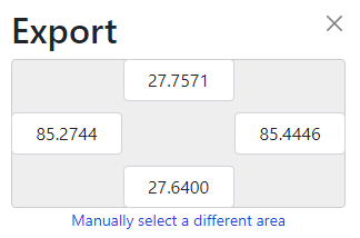
Map extent coordinates On the right side of the website you can see the extent of map selected like this image.

Map extent Export supports only small amount of data. Therefore you need to click the link to Overpass API. This will start downloading the data which you can display on the map.
You need to convert the projection of road data to UTM.
As explained, you can also download vector data as Geopackage from this link.
4.3.1.2 Export the necessary data only
In the data, downloaded from above link, there are some road links which are not accessible. Therefore, we will select by attribute and export only those features which are required for this analysis. In the Select by Expression tool use the following expression.
highway = 'primary' or
 highway = 'road' or
 highway = 'secondary' or
 highway = 'tertiary' or
highway =  'trunk' or
highway = 'residential' or
name is not NULL
Export the selected features to new layer(roads) in a new Geopackage file (e.g. nw-practice.gpkg). Show the newly created layer in the canvas and remove other layers.
4.3.1.3 Add speed field using following expression in the field calculator
CASE
WHEN highway='trunk' THEN 80
WHEN highway='primary' THEN  60
WHEN highway='secondary' THEN  40
WHEN highway='tertiary' THEN  30
WHEN highway='road' THEN  30
WHEN highway='residential' THEN 20
ELSE 10
END
4.3.1.4 Create nodes
We will use node as a starting point from which we will find the service area. Use the processing tool v.to.points and create nodes at 500m interval. Choose the output file as a layer (e.g. node) of the nw-practice.gpkg.
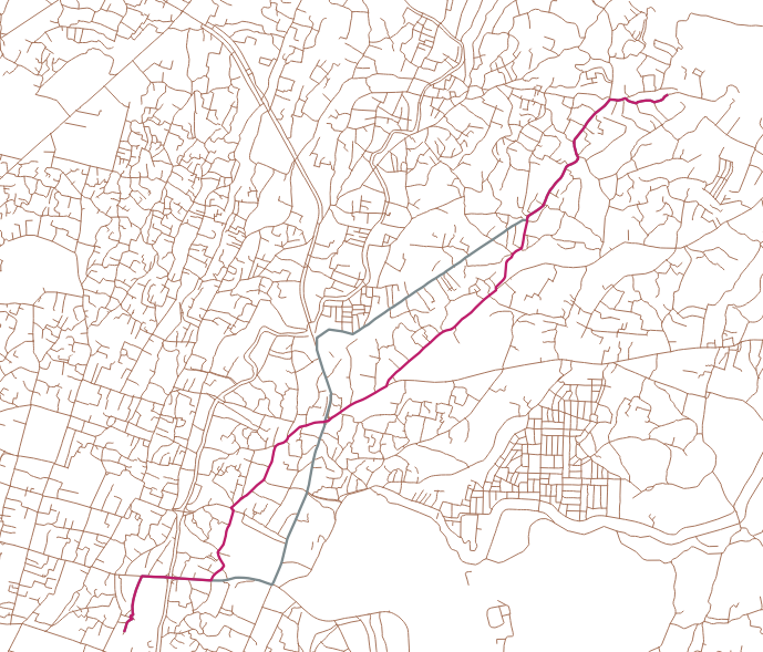
4.3.1.5 Find the shortest path
- Shortest
- Run processing tool Shortest path point-to-point.
- Input vector layer: roads
- Path type: Shortest
- Click button … at Start Point and End Point and select each on the canvas
- Run the tool
- Fastest
- Run processing tool Shortest path point-to-point.
- Input vector layer: roads
- Path type: Fastest
- Speed field: speed
- Click button … at Start Point and End Point and select each on the canvas
- Run the tool
4.3.1.6 Find Service Area
- Shortest
- Run processing tool Service Area From Point.
- Input vector layer: roads
- Path type: Shortest
- Click button … at Start Point and click any node on the canvas
- Run the tool
Fastest
- Run processing tool Service Area From Point.
- Input vector layer: roads
- Path type: Fastest
- Speed field: speed
- Click button … at Start Point and click any node on the canvas
- Run the tool
4.3.2 Steps (practice) for optimization of accessibility (e.g. Garbage container)
- Select a point representing location of Garbage container (and set “selected” attribute to true)
- Find service area from the point
- Select all points on the service area
- Set “removed” attribute to true
- Repeat above process until few points remain
4.3.2.1 Manual/Programming method for above steps
First of all create two extra (boolean) fields (selected and removed) for node layer. Keep the value as false for both the fields for all the features.
Step-1: (Manual)
- Select one of the nodes
- Using field calculator change the value of selected to true (Note: Only for selected feature)
Step-1: (Programming)
- First of all find the fid (e.g. 500) of the feature to be selected as the location of component
#------------------
# Set Node layer(from the list of displayed layers)
ptlayer = QgsProject.instance().mapLayersByName('node')[0]
# Set network layer
vl = QgsProject.instance().mapLayersByName('roads')[0]
# Select node with fid=500
ptlayer.selectByExpression(f'"fid"=500')

# Start editing the layer
ptlayer.startEditing()
for feat in ptlayer.selectedFeatures():
    ptlayer.changeAttributeValue(feat.id(), 5, True) # Set 5th attribute to true

# End editing and remove selection
ptlayer.commitChanges()
ptlayer.removeSelection()
# Get the coordinate of the selected point for next step
geom = feat.geometry()
xy = geom.asPoint()
Step-2: Find service area(Manual) - Select service area from point tool - Provide the parameters for tool and run
Step-2 (Program) > Note: All the tools in the processing toolbox has a name which is displayed on hovering the cursor. The name of service area from point tool is native:serviceareafrompoint.
- Define the parameters to be used for the tool
- code for running the tool
#------------------
# Parameters for service area tool
param = {
        'INPUT': vl, # Network layer
        'START_POINT': f'{xy[0]}, {xy[1]}', # Coordinates of selected point
        'TRAVEL_COST2':1500, #Travelled distance
        'OUTPUT_LINES':'TEMPORARY_OUTPUT' # Don't save the output
    }

# Run the tool and save its output in the variable *result*
result = processing.run("native:serviceareafrompoint", param)['OUTPUT_LINES']
# Display the result (We will comment out the following line in the actual loop)
QgsProject.instance().addMapLayer(result)
Step-3: (Manual) Select all the nodes on the service area and set its removed value to true
- Select the tool named Select within distance in the processing tool
- Select features: node, Compare features: service area
- Within: 1.0 (m)
- Run the tool
- Edit and change the removed attribute of selected nodes to true
Step-3: Program
- Define parameters
- Run tool
#------------------
# Parameters for select-within-distance tool
parampt = {
'INPUT': ptlayer,
'REFERENCE': result,
'DISTANCE': 1.0
}
# Run the tool
processing.run("native:selectwithindistance", parampt)
# Edit the *removed* attribute
ptlayer.startEditing()
for feat in ptlayer.selectedFeatures():
ptlayer.changeAttributeValue(feat.id(), 6, True)
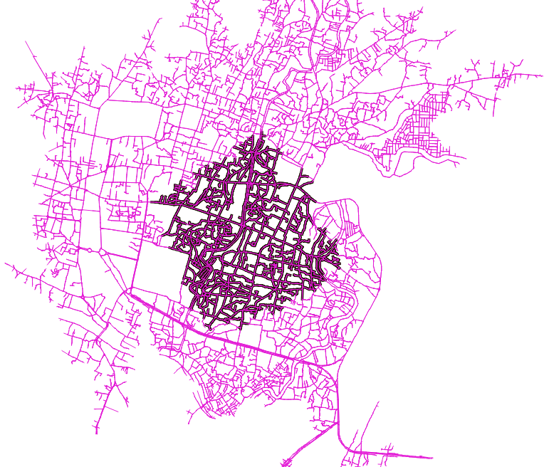
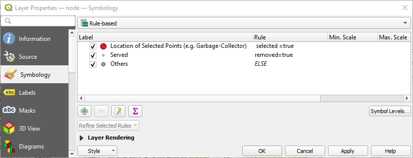
ptlayer.commitChanges()4.3.2.2 Visualization of Results
- Change the symbology as below to make the display more clear
After Running the following full code (combined from above) twice we get the results shown below the codes.
#------------------

# Set Node layer(from the list of displayed layers)
ptlayer = QgsProject.instance().mapLayersByName('node')[0]
# Set network layer
vl = QgsProject.instance().mapLayersByName('roads')[0]
# Select node with fid=500
ptlayer.selectByExpression(f'"fid"=500')

# Start editing the layer
ptlayer.startEditing()
for feat in ptlayer.selectedFeatures():
    ptlayer.changeAttributeValue(feat.id(), 5, True) # Set 5th attribute to true

# End editing and remove selection
ptlayer.commitChanges()
ptlayer.removeSelection()
# Get the coordinate of the selected point for next step
geom = feat.geometry()
xy = geom.asPoint()
# Parameters for service area tool
param = {
        'INPUT': vl, # Network layer
        'START_POINT': f'{xy[0]}, {xy[1]}', # Coordinates of selected point
        'TRAVEL_COST2':1500, #Travelled distance
        'OUTPUT_LINES':'TEMPORARY_OUTPUT' # Don't save the output
    }

# Run the tool and save its output in the variable *result*
result = processing.run("native:serviceareafrompoint", param)['OUTPUT_LINES']
# Display the result (We will comment out the following line in the actual loop)
QgsProject.instance().addMapLayer(result)
# Parameters for select-within-distance tool
parampt = {
    'INPUT': ptlayer,
    'REFERENCE': result,
    'DISTANCE': 1.0
}

# Run the tool
processing.run("native:selectwithindistance", parampt)
# Edit the *removed* attribute
ptlayer.startEditing()
for feat in ptlayer.selectedFeatures():
     ptlayer.changeAttributeValue(feat.id(), 6, True)

ptlayer.commitChanges()
4.3.2.3 Finally
We can loop the whole code by selecting the point-layer feature randomly or in a sequence.
5 Summary
We learned:
- General use of python
- What is a python variable
- String, integer and float
- About range, list, tuple and dictionary
- How to print the value of a variable
- Operations involving string and numbers
- If statement, for and while loops
- Using python in QGIS
- Accessing GIS data layers
- Loading vector and raster layers to the map
- Accessing features and attributes of vector layer
- Using python code for service area optimization
- How to edit the layer attribute
- How to set parameter for a processing tool
- How to run a processing tool