| time(seconds) | length | speed(km/hr) | turtuosity | Elevation difference |
|---|---|---|---|---|
| 51.00 | 54 | 29 | 30.00 | 29 |
| 500.00 | 500 | 500 | 500.00 | 500 |
| 36.00 | 33 | 63 | 59.00 | 63 |
| 1.16 | 1 | 1 | 1.00 | 1 |
| 17.00 | 19 | 1 | 8.00 | 9 |
| 38.00 | 23 | 29 | 153.00 | 31 |
| 500.00 | 500 | 500 | 500.00 | 500 |
| 48.00 | 78 | 63 | 12.00 | 57 |
| 1.00 | 1 | 1 | 1.05 | 1 |
| 14.00 | 9 | 6 | 18.00 | 13 |
Abstract
GNSS based location tracking was done from Kathmandu to Biratnagar via Sindhuli Road. Private passenger microbus running from Kathmandu to Biratnagar was used for travel. The total tracked length was divided into 500m sections and an analysis was done to understand the relation between the speed, absolute elevation difference and turtuosity of the road sections.
Introduction
Recently most of the mobile phones come equipped with location tracking (GNSS) devices. There are plenty of freely available apps which can record the location and speed of the device while moving. One of the apps called “OSMTracker” was used for the present analysis. OSMTracker is available for android free of cost. It can be used to track the location and add waypoints, photos, audio etc which can be exported and viewed in GIS software. For the purpose of present analysis, QGIS was used for data viewing and R software was used for analysis.
About OSMTracker and gpx
What is OSMTracker?
OSMTracker is a mobile app which tracks your location every second and saves the track as gpx file. The file can be saved to the device or uploaded to the openstreetmap website. We can also add location of favorite places while moving or capture a photograph which will be tagged with the location.
What is gpx?
Full form of gpx is GPS Exchange Format. It is a vector data format which saves multiple vector layers in a single file. QGIS or any GIS software can display the gpx data. Three of the vector layers are described below.
route_points: Point vector data which records all the point (at 1 second interval). Speed and location (x, y, altitude) are recorded.
waypoints: Point vector data which records the point of interest recorded by the user while tracking. Waypoints can have photo, text, audio or many other types of attribute.
track: It is line vector data which represents linear feature from start to the end of the track.
Road From Kathmandu to Biratnagar
There are not so many alternatives to reach Biratnagar from capital city Kathmandu. Two major portions of road used in the present case are: 1) Newly constructed road joining Kathmandu with the plane area of Nepal (Popularly known as Banepa Sindhuli Bardibas road and 2) East-West highway joining eastern extreme to western extreme of southern plane of Nepal. The first portion is narrow (4m) mountain road and the next one is wide and passes through flat terrain.
Banepa Sindhuli Bardibas Road
This road was completed recently with the aid of Japanese government and handed over to Nepal government just after the famous earthquake of 12th April, 2015. The road passes through scenic mountains of Nepal mid hills and lower hills confronting Terai planes. At numerous locations the road passes through highly tortuous route with continuous hairpin bends. Breathtaking structures comprising heavy cuttings supported by high retaining walls constructed partly with stone filled gabions are one of the major component of the road. Road side channels, well maintained road surface and some heavy hill side protection works have become major attraction. One such protection work named as ‘Selfie-danda’ or ‘Selfie hill’ about few kilometers from Sindhuli has become hallmark of the road.
Following image shows Kathmandu to Bardibas section of road.
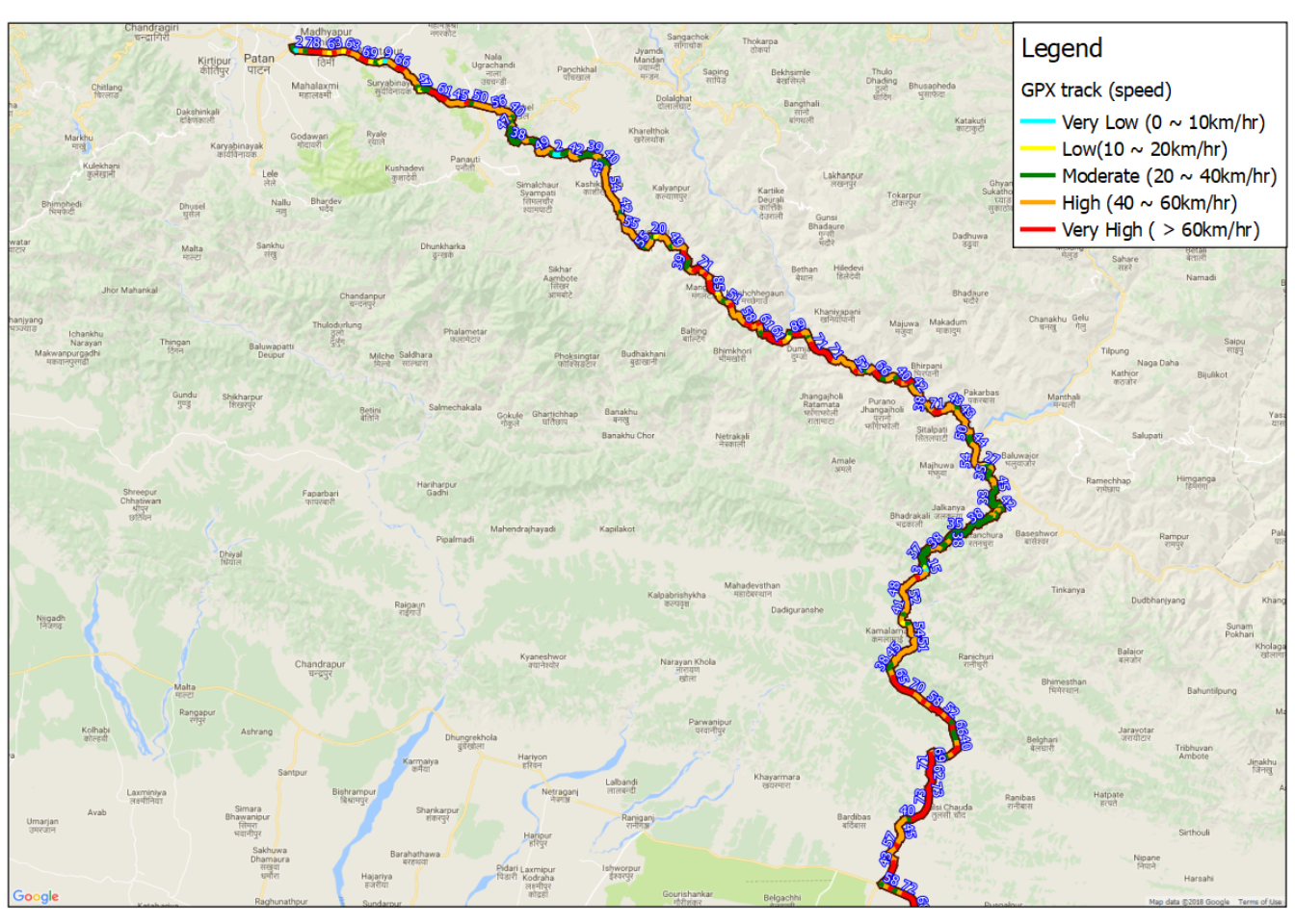
East West Highway
It is one of the oldest highway of Nepal constructed around 40 years back. Most part of the road passes through plane Terai area. Roads are generally well maintained and wide.
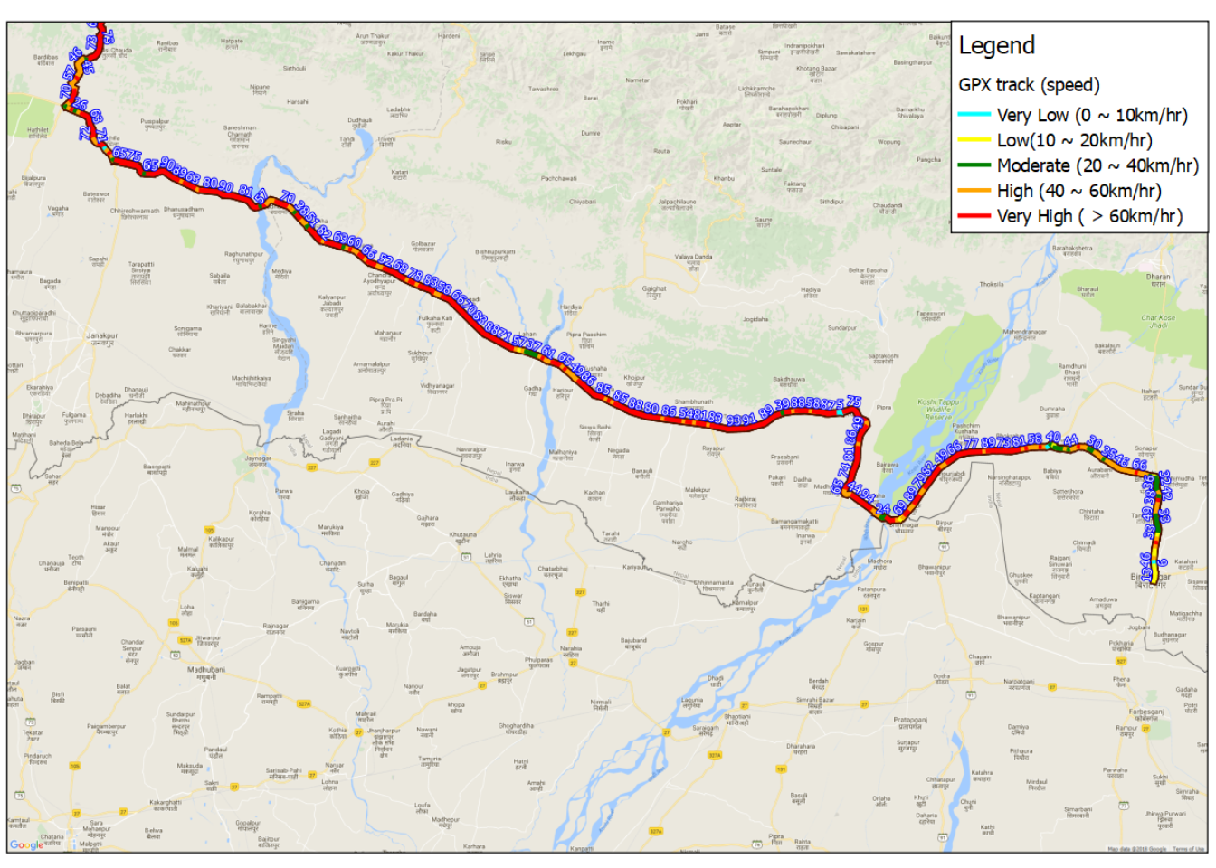
Bardibas to Kathmandu is shown in figure below.
Methodology
The speed of vehicle depends mainly on following factors
- Condition of road
- Elevation difference (If the road has many ups and downs the speed will be low)
- Turtuosity: Road curves restrict the speed of vehicle.
- Driver: Each driver has their own driving skill and attitude which affects the speed. In general, private vehicle drivers in Nepal tend to drive at higher speed.
For the current study only two factors were counted as follows:
Sum of absolute elevation difference: Absolute elevation difference at each recorded location was added for up to 500m length
Turtuosity: it is defined as the length of the road section divided by the straight distance between the starting point and the end point. Following figure illustrates the concept of turtuosity.
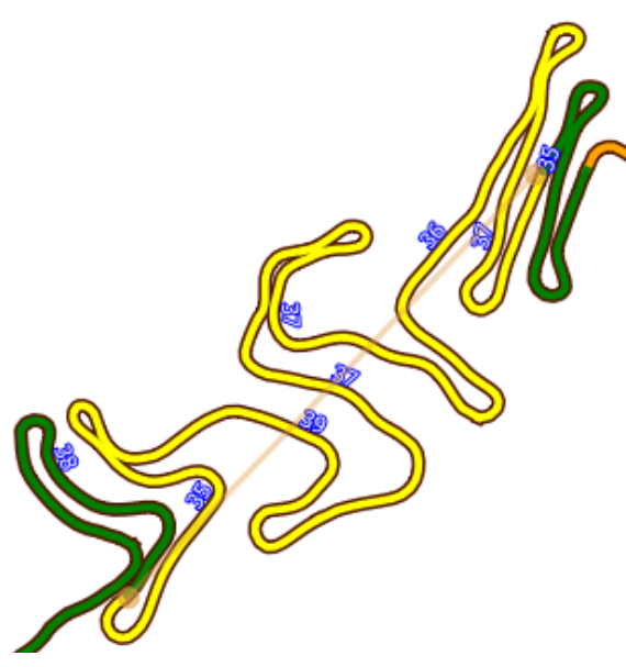
In this figure the actual road length along the road in yellow color is 3.0km while the actual point to point distance is about 580m. Therefore the turtuosity will be calculated as follows:
\[ turtuosity = \frac{3.0}{0.58} = 5.2 \]
TheOSMTracker records the location at one-second interval. At a speed of 30km-per-hour it covers almost 10m in one second. At each location it also record elevation. Total elevation difference for 500km can be expressed by following equation.
\[ \Delta{El} = \sum{|\delta{El}|} \]
Data analysis
Multivariate statistical analysis was performed in ‘R’ to calculate the relation between vehicle speed and the two parameter (elevation difference and turtuosity). Following code gives the relation.
rm(list = ls())
library(rgdal)
shape <- readOGR(dsn = "path/to/shapefile", layer = "tracksp")
shape.s1 <- shape[shape$turtuosity<3.0 & shape$speed>20.0,]
# plot(shape.s1$speed, shape.s1$turtuosity)
dt <- cbind(shape.s1$speed, shape.s1$turtuosity, shape.s1$elevdif)
lmreg <- lm(speed ~ turtuosity + sqrt(elevdif), data=shape.s1)
sp1 <- lmreg$fitted.values[lmreg$fitted.values>0]
sp2 <- shape.s1$speed[lmreg$fitted.values>0]
summary(lmreg) # gives the summary of result
Following equation is obtained from the multivariate analysis. R-squared of the fitted equation is 0.3391 which may be considered low but it can give us a basic idea about the relation.
\[ speed = 95.2 - 19.5 \times turtuosity - 1.05 \times (\Delta{El}) \]
| parameters | Estimate | Std. Error |
|---|---|---|
| Intercept | 95.2349 | 2.5749 |
| turtuosity | -19.46632 | 2.49961 |
| elevdif | -1.0489 | 0.07961 |
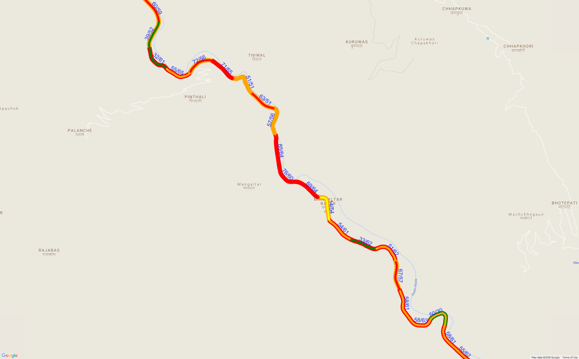
Comparison Speed was recalculated for each section using the fitted equation. Following observations were made (Calculated speed is referred to as ‘proposed speed’):
For around 50% of sections the actual speed was higher than the proposed speed. Same for the opposite. The speed can be higher at some straight sections while for the curves the speed should be kept low.
Highest speed goes to more than 90km/hr while the highest proposed speed is around 75km/hr.
Following figure illustrates the comparison between actual and proposed speed. Outline color of the road shows the proposed speed. The label shows \(speed_{actual}/speed_{proposed}\).
Extra
Following steps were performed to segment the road into 500m sections and to calculate the speed, turtuosity and elevation difference for each section.
- Open QGIS and add vector layer (select the gpx file)
- Select route_points layer
- From ‘Menu->Plugins’ select ‘python console’. Click ‘Show editor’ tool in the console. Copy the following code and paste to the editor. Save file as python (such as:gpx.py) file.
- Run python code from console.
Code
Note: Code shoud be revised for python version-3
from PyQt4.Qt import QVariant
from PyQt4.QtGui import QColor
def getDistance(p1, p2):
    m = d.measureLine(p1, p2)
    m = d.convertMeasurement(m, 2, 0, False)
    return m[0]
def getLineLength(l):
    m = d.measureLength(l)
    m = d.convertMeasurement(m, 2, 0, False)
    return m[0]
def getRadius(pArr, ll):
    pt = []
    pt.append(pArr[0])
    l = len(pArr)
    pt.append(pArr[l-1])
    pline = QgsGeometry.fromPolyline(pt)
    return ll/getLineLength(pline)

def interpolate_pt(p1, p2,  d, d1):
    f = (d - d1)/d
    x1 = p1.x()
    x2 = p2.x()
    y1 = p1.y()
    y2 = p2.y()
    x = x1 + (x2 - x1)*f
    y = y1 + (y2 - y1)*f

    # print x1, x2, d, d1, x, y
    return QgsPoint(x, y)

# create split line
track = iface.activeLayer()

vLyr = QgsVectorLayer('linestring?crs=EPSG:4326','track100','memory')
QgsMapLayerRegistry.instance().addMapLayer(track)
vpr = vLyr.dataProvider()
vpr.addAttributes([QgsField("pid", QVariant.Int),
                   QgsField("time", QVariant.Double),
                   QgsField("length",QVariant.Double),
                   QgsField("speed",QVariant.Double),
                   QgsField("elevdif",QVariant.Double),
                   QgsField("radius", QVariant.Double), # radius ratio
                   QgsField("fspeed", QVariant.Double),
                   QgsField("ftime", QVariant.Double)])
vLyr.updateFields()

feat = track.getFeatures()
trackpt = []
flen = 0.0
for f in feat:
    trackpt.append(f)
npt = len(trackpt)
# starting point (Initial points can be skipped)
fp = 500
# end point (Last few points can be skipped)
ep = 500
#length of each segment
seg = 500.0
p1 = trackpt[fp].geometry().asPoint()
pts = [p1]
j = 0
vF = []
dt = 0
dAlt = 0.0
# coefficients calculated from R analysis
coef = {'elev':-1.049, 'radius':-19.466,'intercept':95.235}
for i in range(fp + 1, npt - ep ):
    d = QgsDistanceArea()
    p2 = trackpt[i   ].geometry().asPoint()
    dist = getDistance(p1, p2)
    flen = flen + dist
    pts.append(p2)
    # time
    tm =( trackpt[i].attribute("time")).toTime_t() - ( trackpt[i -1].attribute("time")).toTime_t()
    dt += tm
    dAlt += abs(trackpt[i].attribute("ele") - trackpt[i -1].attribute("ele") )
    if flen > seg:
        dd = flen - seg
        p1 = interpolate_pt( p1, p2, dist, dd)
        pts.pop()
        pts.append(p1)
        dt = dt - tm + (dd / dist * tm)
        j += 1
        pline = QgsGeometry.fromPolyline(pts)
        flen = getLineLength(pline)
        qf = QgsFeature()
        qf.setGeometry(pline)
        speed = flen /dt * 3.6
        radius = getRadius(pts, flen)
        rad2 = radius
        if rad2 > 2.0:
            rad2 = 2.0
        fspeed = coef['elev']*dAlt + coef['radius']*rad2+coef['intercept']
        ftime = 1800.0 / fspeed
        qf.setAttributes([j, dt, flen, speed, dAlt,radius,fspeed, ftime])
        vF.append(qf)
        # print j, i, flen
        flen = 0
        pts  = [p1]
        i = i -1
        dt = 0
        dAlt = 0.0
    else:
        p1 = p2
vpr.addFeatures(vF)
vLyr.commitChanges()
filename = "path/to/tracksp.shp"
QgsVectorFileWriter.writeAsVectorFormat(vLyr, filename,
                "UTF-8", None, "ESRI Shapefile")

vLyrB =  QgsVectorLayer(filename, "Speed(actual)", "ogr")

vLyr = QgsVectorLayer(filename, "GPX track (speed)", "ogr")
# Render
speedrange = (
("Very Low (0 ~ 10km/hr)", 0.0, 10.0, "cyan"),
("Low(10 ~ 20km/hr)", 10.0001, 20.0, "yellow"),
("Moderate (20 ~ 40km/hr)", 20.0001, 40.0, "green"),
("High (40 ~ 60km/hr)", 40.0001, 60.0, "orange"),
("Very High ( > 60km/hr)", 60.0001, 200.0, "red"))

ranges = []
ranges2 = []
for label, lower, upper, color in speedrange:
    sym = QgsSymbolV2.defaultSymbol(vLyr.geometryType())
    sym.setColor(QColor(color))
    sym.setWidth(0.6)
    rng = QgsRendererRangeV2(lower, upper, sym, label)
    ranges.append(rng)
    sym.setWidth(1.5)
    rng = QgsRendererRangeV2(lower, upper, sym, label)
    ranges2.append(rng)

field = "speed"
renderer = QgsGraduatedSymbolRendererV2(field, ranges)
vLyr.setRendererV2(renderer)
renderer = QgsGraduatedSymbolRendererV2('fspeed', ranges2)
vLyrB.setRendererV2(renderer)
# label

lbl = QgsPalLayerSettings()
lbl.readFromLayer(vLyrB)
lbl.enabled = True
lbl.isExpression = True
lbl.fieldName = "round(\"speed\", 0) || round(\"fspeed\",0)"
lbl.bufferDraw = True
lbl.bufferColor = QColor("blue")
lbl.bufferSize = 0.7
lbl.textColor = QColor("white")
lbl.placement = QgsPalLayerSettings.AboveLine
lbl.setDataDefinedProperty(QgsPalLayerSettings.Size, True, True, '8', ' ')
lbl.writeToLayer(vLyrB)
QgsMapLayerRegistry.instance().addMapLayer(vLyrB)
QgsMapLayerRegistry.instance().addMapLayer(vLyr)
print ("finished")