5 Methodology

The speed of vehicle depends mainly on following factors

Condition of road
Elevation difference (If the road has many ups and downs the speed will be low)
Turtuosity: Road curves restrict the speed of vehicle.
Driver: Each driver has their own driving skill and attitude which affects the speed. In general, private vehicle drivers in Nepal tend to drive at higher speed.

For the current study only two factors were counted as follows:

Sum of absolute elevation difference: Absolute elevation difference at each recorded location was added for up to 500m length
Turtuosity: it is defined as the length of the road section divided by the straight distance between the starting point and the end point. Following figure illustrates the concept of turtuosity.

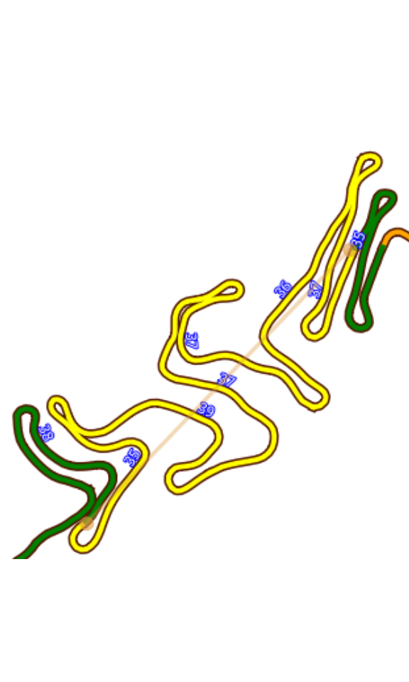
Figure 5.1: Concept of Turtuosity

In this figure the actual road length along the road in yellow color is 3.0km while the actual point to point distance is about 580m. Therefore the turtuosity will be calculated as follows:

\[\begin{equation} turtuosity = \frac{3.0}{0.58} = 5.2 \end{equation}\]

TheOSMTracker records the location at one-second interval. At a speed of 30km-per-hour it covers almost 10m in one second. At each location it also record elevation. Total elevation difference for 500km can be expressed by following equation.

\[\begin{equation} \Delta{El} = \sum{|\delta{El}|} \end{equation}\]

where \(\Delta{El}\) is total elevation difference for 500m stretch, and \(\delta{El}\) is the elevation difference at each location record.

We get the following table (Table 5.1) of values.

Table 5.1: Compiled values of turtuosity and elevation difference
time(seconds)	length	speed(km/hr)	turtuosity	Elevation difference
51	500	36	1.16	17
38	500	48	1.00	14
54	500	33	1.00	19
23	500	78	1.00	9
29	500	63	1.00	1
29	500	63	1.00	6
30	500	59	1.00	8
153	500	12	1.05	18
29	500	63	1.00	9
31	500	57	1.00	13

5.1 Data compilation

Route point layer of GPX data was displayed in QGIS, and the parameters (elevation difference and turtuosity) were calculated for each 500m section using python program. The python code is in the last chapter of the report. It may need some changes according to the drive paths and variable choice.

5.2 Data analysis

Multivariate statistical analysis was performed in ‘R’ to calculate the relation between vehicle speed and the two parameter (elevation difference and turtuosity). Following code gives the relation.

rm(list = ls())
library(rgdal)
shape <- readOGR(dsn = "path/to/shapefile", layer = "tracksp")
shape.s1 <- shape[shape$turtuosity<3.0 & shape$speed>20.0,]
# plot(shape.s1$speed, shape.s1$turtuosity)
dt <- cbind(shape.s1$speed, shape.s1$turtuosity, shape.s1$elevdif)
lmreg <- lm(speed ~ turtuosity + sqrt(elevdif), data=shape.s1)
sp1 <- lmreg$fitted.values[lmreg$fitted.values>0]
sp2 <- shape.s1$speed[lmreg$fitted.values>0]
summary(lmreg) # gives the summary of result

Following equation is obtained from the multivariate analysis. R-squared of the fitted equation is 0.3391 which may be considered low but it can give us a basic idea about the relation.

\[\begin{equation} speed = 95.2-19.5*turtuosity - 1.05*(\Delta{El}) \end{equation}\]

Summary of the analysis of result is shown below.

Table 5.2: Summary of coefficients and error
parameters	Estimate	Std. Error
Intercept	95.23490	2.57490
turtuosity	-19.46632	2.49961
elevdif	-1.04890	0.07961

5.3 Comparison

Speed was recalculated for each section using the fitted equation. Following observations were made (Calculated speed is referred to as ‘proposed speed’):

For around 50% of sections the actual speed was higher than the proposed speed. Same for the opposite. The speed can be higher at some straight sections while for the curves the speed should be kept low.
Highest speed goes to more than 90km/hr while the highest proposed speed is around 75km/hr.

Following figure (Fig. 5.2) illustrates the comparison between actual and proposed speed. Outline color of the road shows the proposed speed. The label shows \(actual_{speed}/proposed_{speed}\).

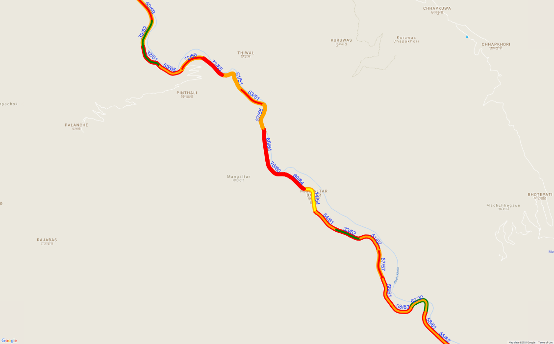
Figure 5.2: Actual vs proposed speed